Mapping and Plotting Precipitation with R

Really interested in quantifying and visualizing weather data for specific areas that we are working…. Here is a first start.

WARNING - this work is stolen!! I have adapted this from a repository on GitHub from the wonderfully talented Milos Popovic. All credit to Milos! What a boss - really awesome stuff.

Also of note is the image used for the blog. That is Cotey Gallagher… I hope she doesn’t sue me. https://www.linkedin.com/pulse/how-crazy-would-could-really-rain-cats-dogs-cotey-gallagher/

First thing we will do is load our packages. If you do not have the packages installed yet you can change the update_pkgs param in the yml of this file to TRUE. Using pak is great because it allows you to update your packages when you want to.

pkgs_cran <- c(
  "here",
  "fs",
  "pRecipe",
  "giscoR",
  "terra",
  "tidyverse",
  "rayshader",
  "sf",
  "classInt",
  "rgl")

pkgs_gh <- c(
  "poissonconsulting/pgfeatureserv",
  "poissonconsulting/fwapgr",
  "NewGraphEnvironment/rfp"
  # we will turn this off since the function it uses won't run for folks without db credentials
  # "NewGraphEnvironment/fpr"
 )

pkgs <- c(pkgs_cran, pkgs_gh)

if(params$update_pkgs){
  # install the pkgs
  lapply(pkgs,
         pak::pkg_install,
         ask = FALSE)
}

# load the pkgs
pkgs_ld <- c(pkgs_cran,
             basename(pkgs_gh))
invisible(
  lapply(pkgs_ld,
       require,
       character.only = TRUE)
)

Define our Area of Interest

Here we diverge a bit from Milos version as we are going to load a custom area of interest. We will be connecting to our remote database using Poisson Consulting’s fwapgr::fwa_watershed_at_measure function which leverages the in database FWA_WatershedAtMeasure function from Simon Norris’ wonderful fwapg package.

We use a blue line key and a downstream route measure to define our area of interest which is the Neexdzii Kwa (a.k.a Upper Bulkley River) near Houston, British Columbia.

As per the Freshwater Atlas of BC - the blue line key:

Uniquely identifies a single flow line such that a main channel and a secondary channel with the same watershed code would have different blue line keys (the Fraser River and all side channels have different blue line keys).

A downstream route measure is:

The distance, in meters, along the route from the mouth of the route to the feature. This distance is measured from the mouth of the containing route to the downstream end of the feature.

# lets build a custom watersehed just for upstream of the confluence of Neexdzii Kwa and Wetzin Kwa
# blueline key
blk <- 360873822
# downstream route measure
drm <- 166030.4

aoi <- fwapgr::fwa_watershed_at_measure(blue_line_key = blk, 
                                        downstream_route_measure = drm) |> 
  sf::st_transform(4326)

Retrieve the Precipitation Data

For this example we will retrieve our precipitation data from Multi-Source Weighted-Ensemble Precipitation using the pRecipe package.

# let's create our data directory
dir_data <- here::here('posts', params$post_dir_name, "data")

fs::dir_create(dir_data)

To actually download the data we are going to put a chunk option that allows us to just execute the code once and update it with the update_gis param in our yml. We will use usethis::use_git_ignore to add the data to our .gitignore file so that we do not commit that insano enourmouse file to our git repository.

pRecipe::download_data(
    dataset = "mswep",
    path = dir_data,
    domain = "raw",
    timestep = "yearly"
)

usethis::use_git_ignore(paste0('posts/', params$post_dir_name, "/data/*"))

Now we read in our freshly downloaded .nc file and clip to our area of interest.

# get the name of the file with a .nc at the end
nc_file <- fs::dir_ls(dir_data, glob = "*.nc")

mswep_data <- terra::rast(
  nc_file
) |>
terra::crop(
    aoi
)

Next we extract the years of the data from the filename of the .nc file and then transform the data into a dataframe. We need to remove the data from 2023 because it is only for January as per the filename:

mswep_tp_mm_global_197902_202301_025_yearly.nc

# the names of the datasets are arbitrary (precipitation_1:precipitation_45) 
# we will rename the datasets to the years.  
# here we extract 2023 from the nc_file name of the file using regex
year_end <- as.numeric(stringr::str_extract(basename(nc_file), "(?<=_\\d{6}_)\\d{4}"))
year_start <- as.numeric(stringr::str_extract(basename(nc_file), "(?<=_)[0-9]{4}(?=[0-9]{2}_[0-9]{6}_)"))

# assign the names to replace 
names(mswep_data) <- year_start:year_end


mswep_df <- mswep_data |>
    as.data.frame(xy = TRUE) |>
    tidyr::pivot_longer(
        !c("x", "y"),
        names_to = "year",
        values_to = "precipitation"
    ) |> 
  # 2023 is not complete so we remove it
    dplyr::filter(year != 2023)

Get Additional Data

We could use some data for context such as major streams, highways and the railway. We get the streams and railway from data distribution bc api using the bcdata package. Our rfp package calls just allow some extra sanity checks on the bcdata::bcdc_query_geodata function. It’s not really necessary but can be helpful when errors occur (ex. the name of the column to filter on is input incorrectly).

# grab all the railways
l_rail <- rfp::rfp_bcd_get_data(
    bcdata_record_id = stringr::str_to_upper("whse_basemapping.gba_railway_tracks_sp")
) |> 
  sf::st_transform(4326) |> 
  janitor::clean_names() 

# streams in the bulkley and then filter to just keep the big ones
l_streams <- rfp::rfp_bcd_get_data(
  bcdata_record_id = stringr::str_to_upper("whse_basemapping.fwa_stream_networks_sp"),
  col_filter = stringr::str_to_upper("watershed_group_code"),
  col_filter_value = "BULK",
  # grab a smaller object by including less columns
  col_extract = stringr::str_to_upper(c("linear_feature_id", "stream_order"))
) |> 
  sf::st_transform(4326) |> 
  janitor::clean_names() |> 
  dplyr::filter(stream_order > 4)

Because the highways we use in our mapping are not available for direct download from the Data Distribution BC api (some other versions are here we will query them from our remote database. The function used (fpr::fpr_db_query) is a wrapper around the DBI::dbGetQuery function that allows us to query our remote database by calling our environmental variables and making a connection. This will not work without the proper credentials so if you were trying to reproduce this and don’t have the credentials you won’t be able to retrieve the roads. To get around this we have stored the trimmed roads data in the data directory of this post so we can read it in from there.

# highways
# define the type of roads we want to include using the transport_line_type_code. We will include RA1 and RH1 (Road arerial/highway major)
rd_codes <- c("RA1", "RH1")
l_rds <- fpr::fpr_db_query(
  query = glue::glue("SELECT transport_line_id, structured_name_1, transport_line_type_code, geom FROM whse_basemapping.transport_line WHERE transport_line_type_code IN ({glue::glue_collapse(glue::single_quote(rd_codes), sep = ', ')})")
  )|> 
  sf::st_transform(4326) 


sf::st_intersection(l_rds, 
                    # we will remove all the aoi columns except the geometry so we don't get all the aoi columns appended
                    aoi |> dplyr::select(geometry)) |> 
  sf::st_write(here::here('posts', params$post_dir_name, "data", "l_rds.gpkg"), delete_dsn = TRUE)

Now we trim up all those layers. We have some functions to validate and repair geometries and then we clip them to our area of interest.

# we don't actually need to trim the rds since we already did that but for simplicity we will do it again
  l_rds <- sf::st_read(here::here('posts', params$post_dir_name, "data", "l_rds.gpkg"), quiet = TRUE) 


layers_to_trim <- tibble::lst(l_rail, l_streams, l_rds)

# Function to validate and repair geometries
validate_geometries <- function(layer) {
  layer <- sf::st_make_valid(layer)
  layer <- layer[sf::st_is_valid(layer), ]
  return(layer)
}

# Apply validation to the AOI and layers
aoi <- validate_geometries(aoi)
layers_to_trim <- purrr::map(layers_to_trim, validate_geometries)

# clip them  with purrr and sf
layers_trimmed <- purrr::map(
  layers_to_trim,
  ~ sf::st_intersection(.x, aoi)
) 

Plot the Precipitation Data by Year

First thing we do here is highjack the plot function from Milos.

theme_for_the_win <- function(){
    theme_minimal() +
    theme(
        axis.line = element_blank(),
        axis.title.x = element_blank(),
        axis.title.y = element_blank(),
        axis.text.x = element_blank(),
        axis.text.y = element_blank(),
        legend.position = "right",
        legend.title = element_text(
            size = 11, color = "grey10"
        ),
        legend.text = element_text(
            size = 10, color = "grey10"
        ),
        panel.grid.major = element_line(
            color = NA
        ),
        panel.grid.minor = element_line(
            color = NA
        ),
        plot.background = element_rect(
            fill = NA, color = NA
        ),
        legend.background = element_rect(
            fill = "white", color = NA
        ),
        panel.border = element_rect(
            fill = NA, color = NA
        ),
        plot.margin = unit(
            c(
                t = 0, r = 0,
                b = 0, l = 0
            ), "lines"
        )
    )
}

breaks <- classInt::classIntervals(
    mswep_df$precipitation,
    n = 5,
    style = "equal"
)$brks

colors <- hcl.colors(
    n = length(breaks),
    palette = "Temps",
    rev = TRUE
)

Now we plot the data by year.

map1 <- ggplot(
    data = mswep_df
) +
geom_raster(
    aes(
        x = x,
        y = y,
        fill = precipitation
    )
) +
geom_contour(
    aes(
       x = x,
       y = y,
       z = precipitation
    ), color = "white" # add this line
) +
geom_sf(
    data = aoi,
    fill = "transparent",
    color = "grey10",
    size = .5
) +
scale_fill_gradientn(
    name = "mm",
    colors = colors,
    breaks = breaks,
    labels = round(breaks, 0), # use round(breaks, 0)
    limits = c(
        min(mswep_df$precipitation),
        max(mswep_df$precipitation)
    )
) +
facet_wrap(~year) +
guides(
    fill = guide_colourbar(
        direction = "vertical",
        barheight = unit(50, "mm"),
        barwidth = unit(5, "mm"),
        title.position = "top",
        label.position = "right",
        title.hjust = .5,
        label.hjust = .5,
        ncol = 1,
        byrow = FALSE
    )
) +
theme_for_the_win()

map1

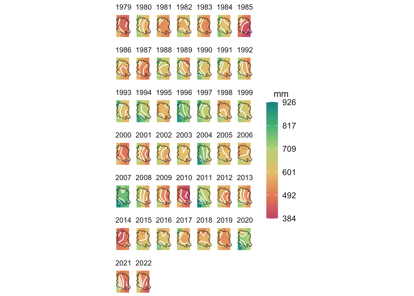
Pretty cool. Interesting to see really wet and dry years in the last 20 years or so such as the wet ones in 2004, 2007, 2011 and 2020 and the dry ones in 2000, 2010, 2014, 2021 and 2022. The contours on the maps are really interesting as they show the gradients which generally run west to east - but occasionally run south to north.

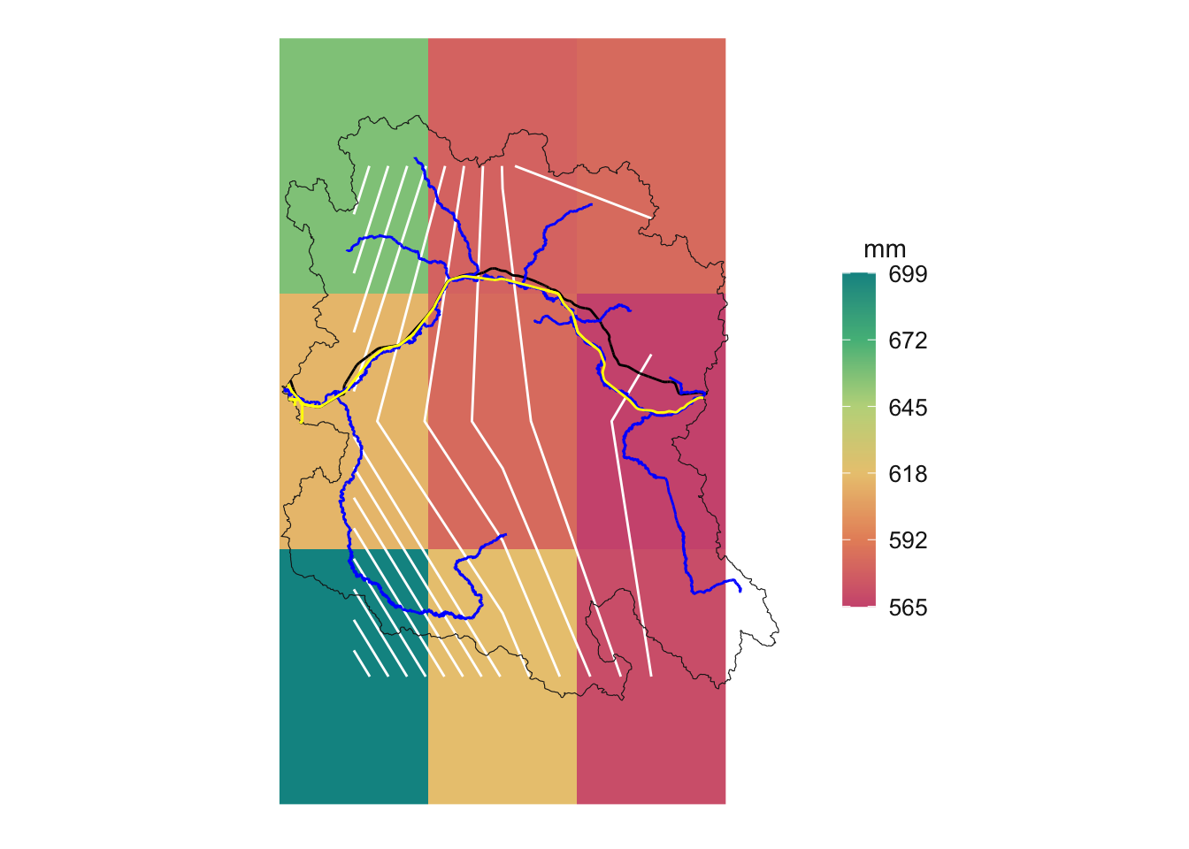
Average Precipitation

Now we will average all the years together to get an average precipitation map. We will add our additional layers for context too. Roads are black, railways are yellow and streams are blue.

mswep_average_df <- mswep_df |>
  dplyr::group_by(
    x, y, .drop = FALSE
  ) |>
  dplyr::summarise(
    precipitation = mean(precipitation)
  ) |> 
  dplyr::mutate(year = "average")


breaks <- classInt::classIntervals(
  mswep_average_df$precipitation,
  n = 5,
  style = "equal"
)$brks


colors <- hcl.colors(
  n = length(breaks),
  palette = "Temps",
  rev = TRUE
)

map_average <- ggplot(
  data = mswep_average_df
) +
  geom_raster(
    aes(
      x = x,
      y = y,
      fill = precipitation
    )
  ) +
  geom_contour(
    aes(
      x = x,
      y = y,
      z = precipitation
    ), color = "white" # add this line
  ) +
  geom_sf(
    data = aoi,
    fill = "transparent",
    color = "grey10",
    size = .5
  ) +
  scale_fill_gradientn(
    name = "mm",
    colors = colors,
    breaks = breaks,
    labels = round(breaks, 0), # use round(breaks, 0)
    limits = c(
      min(mswep_average_df$precipitation),
      max(mswep_average_df$precipitation)
    )
  ) +
  guides(
    fill = guide_colourbar(
      direction = "vertical",
      barheight = unit(50, "mm"),
      barwidth = unit(5, "mm"),
      title.position = "top",
      label.position = "right",
      title.hjust = .5,
      label.hjust = .5,
      ncol = 1,
      byrow = FALSE
    )
  ) +
  geom_sf(
    data = layers_trimmed$l_rds,
    color = "black",
    size = .8
  ) +
  geom_sf(
    data = layers_trimmed$l_streams,
    color = "blue",
    size = .8
  ) +
  geom_sf(
    data = layers_trimmed$l_rail,
    color = "yellow",
    size = .8
  ) +
  theme_for_the_win()

map_average

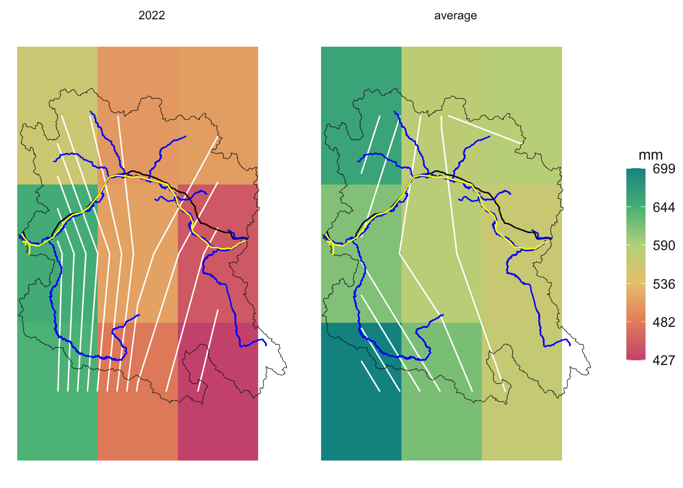
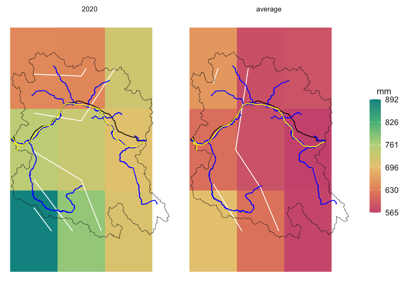
Compare the Average Precipitation to a Specific Year

We often talk about a “dry” year or a “wet” year. Let’s compare the average precipitation to a specific year. We will build a little function to do this so that we can easily compare any year to the average.

map_vs_average <- function(year_compare){
  
  mswep_df_2022 <- mswep_df |>
    dplyr::filter(year == year_compare) |> 
    dplyr::mutate(year = as.character(year))
  
  mswep_df_compare <- bind_rows(mswep_average_df, mswep_df_2022)
  
  breaks <- classInt::classIntervals(
    mswep_df_compare$precipitation,
    n = 5,
    style = "equal"
  )$brks
  
  colors <- hcl.colors(
    n = length(breaks),
    palette = "Temps",
    rev = TRUE
  )
  
  ggplot(
    data = mswep_df_compare
  ) +
    facet_wrap(~year) +
    geom_raster(
      aes(
        x = x,
        y = y,
        fill = precipitation
      )
    ) +
    geom_contour(
      aes(
        x = x,
        y = y,
        z = precipitation
      ), color = "white" # add this line
    ) +
    geom_sf(
      data = aoi,
      fill = "transparent",
      color = "grey10",
      size = .5
    ) +
    scale_fill_gradientn(
      name = "mm",
      colors = colors,
      breaks = breaks,
      labels = round(breaks, 0), # use round(breaks, 0)
      limits = c(
        min(mswep_df_compare$precipitation),
        max(mswep_df_compare$precipitation)
      )
    ) +
    guides(
      fill = guide_colourbar(
        direction = "vertical",
        barheight = unit(50, "mm"),
        barwidth = unit(5, "mm"),
        title.position = "top",
        label.position = "right",
        title.hjust = .5,
        label.hjust = .5,
        ncol = 1,
        byrow = FALSE
      )
    ) +
    geom_sf(
      data = layers_trimmed$l_rds,
      color = "black",
      size = .8
    ) +
    geom_sf(
      data = layers_trimmed$l_streams,
      color = "blue",
      size = .8
    ) +
    geom_sf(
      data = layers_trimmed$l_rail,
      color = "yellow",
      size = .8
    ) +
    theme_for_the_win()
}

First let’s check out 2022 as it seemed pretty dry.

map_vs_average(2022)

Now let’s look at 2020 as that seemed wet with lots of streams flowing really nicely.

map_vs_average(2020)

Definitely wetter than average.

3D Contour Map

Let’s make an interactive 3D contour map of the average precipitation data. Use the mouse to rotate the map and zoom in and out!

{
  
  rayshader::plot_gg(
    ggobj = map_average,
    width = 7,
    height = 7,
    scale = 250,
    solid = FALSE,
    shadow = TRUE,
    shadowcolor = "white",
    shadowwidth = 0,
    shadow_intensity = 1,
    # window.size = c(600, 600),
    zoom = .7,
    phi = 30,
    theta = 337.5
    # fov =30
  )
  rgl::rglwidget(width = 982, height = 1025, reuse = FALSE)
}

Thanks Miles!