Getting details of historic orthophoto imagery with R

We would like to obtain historic ortho photo imagery so that we can compare historic watershed conditions compared to current (ex. floodplain vegetation clearing, channel morphology, etc.). For our use case — restoration baseline condition assessment and impact evaluation of land cover change — our goal is to reconstruct historical conditions for entire sub-basins, as far back as possible (e.g., 1930 or 1960), and programmatically compare these to recent remotely sensed land cover analysis.

Code

suppressMessages(library(tidyverse))
library(ggplot2)
library(bcdata)
library(fwapgr)
library(knitr)
suppressMessages(library(sf))
library(crosstalk)
library(leaflet)
library(leafem)
library(DT)
library(htmltools)

Code

path_post <- fs::path(
  here::here(),
  "posts",
  params$post_name
)

Code

staticimports::import(
  dir = fs::path(
    path_post,
    "scripts"
  ),
  outfile = fs::path(
    path_post,
    "scripts",
    "staticimports",
    ext = "R"
  )
)

Code

source(
  fs::path(
    path_post,
    "scripts",
    "staticimports",
    ext = "R"
  )
)


lfile_name <- function(dat_name = NULL, ext = "geojson") {
  fs::path(
    path_post,
    "data",
    paste0(dat_name, ".", ext)
  )
}

lburn_sf <- function(dat = NULL, dat_name = NULL) {
  if (is.null(dat_name)) {
    cli::cli_abort("You must provide a name for the GeoJSON file using `dat_name`.")
  }
  
  dat |>
    sf::st_write(
      lfile_name(dat_name),
      delete_dsn = TRUE
      # append = FALSE
    )
}

# Function to validate and repair geometries
lngs_geom_validate <- function(layer) {
  layer <- sf::st_make_valid(layer)
  layer <- layer[sf::st_is_valid(layer), ]
  return(layer)
}

Code

# definet he buffer in m
buf <- 1500

Generate an Area of Interest

Here we download our area of interest which is the Neexdzii Kwah River (a.k.a Upper Bulkley River) which is located between Houston, BC (just south of Smithers) and Topley, BC which is east of Houston and north of Burns Lake, BC. We hit up our remote database managed by Simon Norris with a package built by Poisson Consulting specifically for the task. We use the downstream_route_measure of the Bulkley River (identified through a unique blue_line_key) to query the watershed area upstream of the point where the Neexdzii Kwah River enters the Wedzin Kwah River (a.k.a Morice River). Since photopoint centres that fall just outside of the watershed can provide imagery of the edge areas of the watershed we buffer this area to an amount that we approximate is half the width or hieght of the ground distance captured by each image (1500m).

Code

# lets build a custom watersehed just for upstream of the confluence of Neexdzii Kwa and Wetzin Kwa
# blueline key
blk <- 360873822
# downstream route measure
drm <- 166030.4



aoi_raw <- fwapgr::fwa_watershed_at_measure(blue_line_key = blk, 
                                        downstream_route_measure = drm) |> 
  # we put it in utm zone 9 so we can easily buffer using meters
  sf::st_transform(32609) |> 
  dplyr::select(geometry)

aoi <- sf::st_buffer(
  aoi_raw,
  dist = buf
) |> 
  sf::st_transform(4326)


#get the bounding box of our aoi
# aoi_bb <- sf::st_bbox(aoi)

#lets burn this so we don't need to download each time
aoi_raw <- lngs_geom_validate(aoi_raw)
aoi <- lngs_geom_validate(aoi)



# now lets buffer our aoi by 1000m

lburn_sf(
  aoi,
  deparse(substitute(aoi)))

lburn_sf(
  aoi_raw,
  deparse(substitute(aoi_raw)))

# map_aoi <- ggplot() +
#   geom_sf(
#       data = aoi_raw,
#       fill = "transparent",
#       color = "black",
#       linewidth = .5
#   ) +
#   geom_sf(
#       data = aoi,
#       fill = "transparent",
#       color = "red",
#       linewidth = .5
#   ) 
#   
# map_aoi

Download Spatial Data Layers From BC DAta Catalogue

Next we grab a few key layers from the BC Data Catalogue API using convenience function from our rfp package (“Reproducable Field Products”) which wrap the provincially maintained bcdata package. We grab:

Railways
Streams in the Bulkley Watershed group that are 4th order or greater.
Orthophoto Tile Polygons
Historic Imagery Points
Historic Imagery Polygons
NTS 1:50,000 Grid (we will see why in a second)
Air Photo Centroids

Code

# grab all the railways
l_rail <- rfp::rfp_bcd_get_data(
    bcdata_record_id = "whse_basemapping.gba_railway_tracks_sp"
) |> 
  sf::st_transform(4326) |> 
  janitor::clean_names() 


# streams in the bulkley and then filter to just keep the big ones
l_streams <- rfp::rfp_bcd_get_data(
  bcdata_record_id = "whse_basemapping.fwa_stream_networks_sp",
  col_filter = "watershed_group_code",
  col_filter_value = "BULK",
  # grab a smaller object by including less columns
  col_extract = c("linear_feature_id", "stream_order", "gnis_name", "downstream_route_measure", "blue_line_key", "length_metre")
) |> 
  sf::st_transform(4326) |> 
  janitor::clean_names() |> 
  dplyr::filter(stream_order >= 4)

# historic orthophotos
# WHSE_IMAGERY_AND_BASE_MAPS.AIMG_HIST_INDEX_MAPS_POLY
#https://catalogue.data.gov.bc.ca/dataset/airborne-imagery-historical-index-map-points
l_imagery_tiles <- rfp::rfp_bcd_get_data(
  # https://catalogue.data.gov.bc.ca/dataset/orthophoto-tile-polygons/resource/f46aaf7b-58be-4a25-a678-79635d6eb986
  bcdata_record_id = "WHSE_IMAGERY_AND_BASE_MAPS.AIMG_ORTHOPHOTO_TILES_POLY") |> 
  sf::st_transform(4326) 

l_imagery_hist_pnts <- rfp::rfp_bcd_get_data(
  bcdata_record_id = "WHSE_IMAGERY_AND_BASE_MAPS.AIMG_HIST_INDEX_MAPS_POINT") |> 
  sf::st_transform(4326) 

l_imagery_hist_poly <- rfp::rfp_bcd_get_data(
  bcdata_record_id = "WHSE_IMAGERY_AND_BASE_MAPS.AIMG_HIST_INDEX_MAPS_POLY") |> 
  sf::st_transform(4326) 

l_imagery_grid <- rfp::rfp_bcd_get_data(
  bcdata_record_id = "WHSE_BASEMAPPING.NTS_50K_GRID") |> 
  sf::st_transform(4326)

Following download we run some clean up to ensure the geometry of our spatial files is “valid”, trim to our area of interest and burn locally so that every time we rerun iterations of this memo we don’t need to wait for the download process which takes a little longer than we want to wait.

Code

# get a list of the objects in our env that start with l_
ls <- ls()[stringr::str_starts(ls(), "l_")] 

layers_all <- tibble::lst(
  !!!mget(ls)
)

# Apply validation to the AOI and layers
layers_all <- purrr::map(
  layers_all, 
  lngs_geom_validate
  )

# clip them  with purrr and sf
layers_trimmed <- purrr::map(
  layers_all,
  ~ sf::st_intersection(.x, aoi)
) 

# Burn each `sf` object to GeoJSON
purrr::walk2(
  layers_trimmed,
  names(layers_trimmed),
  lburn_sf
)

Code

# lets use the nts mapsheet to query the photo centroids to avoid a massive file download
col_value <- layers_trimmed$l_imagery_grid |> 
  dplyr::pull(map_tile) 

l_photo_centroids <- rfp::rfp_bcd_get_data(
  bcdata_record_id = "WHSE_IMAGERY_AND_BASE_MAPS.AIMG_PHOTO_CENTROIDS_SP",
  col_filter = "nts_tile",
  col_filter_value = col_value) |> 
  sf::st_transform(4326) 

# Apply validation to the AOI and layers
l_photo_centroids <-lngs_geom_validate(l_photo_centroids)

# clip to aoi - can use  layers_trimmed$aoi 
l_photo_centroids <- sf::st_intersection(l_photo_centroids, aoi)


lburn_sf(l_photo_centroids, "l_photo_centroids")

Next - we read the layers back in. The download step is skipped now unless we turn it on again by changing the update_gis param in our memo yaml header to TRUE.

Code

# now we read in all the sf layers that are local so it is really quick
layers_to_load <- fs::dir_ls(
  fs::path(
    path_post,
    "data"),
  glob = "*.geojson"
)

layers_trimmed <- layers_to_load |>
  purrr::map(
    ~ sf::st_read(
      .x, quiet = TRUE)
  ) |> 
  purrr::set_names(
    nm =tools::file_path_sans_ext(
      basename(
        names(
          layers_to_load
        )
      )
    )
  )

Map the Area of Interest

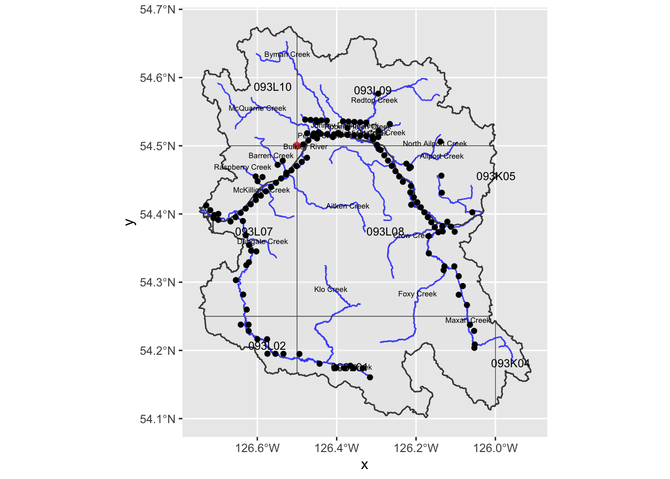
Area of interest is mapped in Figure 1.

Code

map <- ggplot2::ggplot() +
  ggplot2::geom_sf(
      data = layers_trimmed$aoi_raw,
      fill = "transparent",
      color = "black",
      linewidth = .5
  ) +
  ggplot2::geom_sf(
      data = layers_trimmed$aoi,
      fill = "transparent",
      color = "yellow",
      linewidth = .5
  ) +
  ggplot2::geom_sf(
    data = layers_trimmed$l_streams,
    color = "blue",
    size = 1
  ) +
  ggplot2::geom_sf(
    data = layers_trimmed$l_rail,
    color = "black",
    size = 1
  ) +
  ggplot2::geom_sf(
    data = layers_trimmed$l_imagery_hist_pnts,
    color = "red",
    size = 2
  ) +
  # ggplot2::geom_sf(
  #   data = layers_trimmed$l_imagery_hist_poly,
  #   color = "red",
  #   size = 10
  # ) +
  ggplot2::geom_sf(
    data = layers_trimmed$l_imagery_grid,
    alpha = 0.25,
  ) +
  ggplot2::geom_sf_text(
    data = layers_trimmed$l_imagery_grid,
    ggplot2::aes(label = map_tile),
    size = 3  # Adjust size of the text labels as needed
  )

map +
  ggplot2::geom_sf_text(
    data = layers_trimmed$l_streams |> dplyr::distinct(gnis_name, .keep_all = TRUE),
    ggplot2::aes(
      label = gnis_name
    ),
    size = 2  # Adjust size of the text labels as needed
  )

Figure 1: Area of interest. The buffered watershed used for historic airphoto analysis is shown in yellow.

Explore the BC Data Catalouge Imagery Layer Options

Orthophoto Tile Polygons

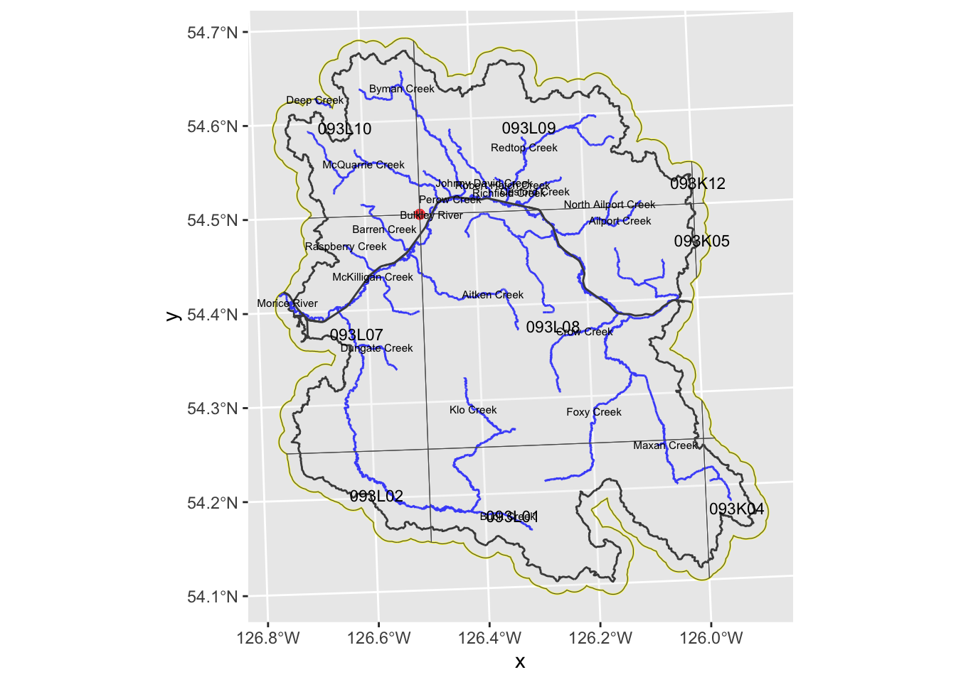
For the Orthophoto Tile Polygons Historic Imagery Polygons layer the range of year_operational is 1996, 2013. This is not as far back as we would prefer to be looking.

Historic Imagery Points

OK, seems we cannot get machine readable historical air photo information from the downloaded from the BC data catalogue Historic Imagery Points layer perhaps because the majority of the photos are not georeferenced? What we see in the map and table below (red dot on map) is one point which contains 8 records including links to pdfs and kmls which are basically a georeferenced drawing of where the imagery overlaps (Table 1 and Figure 2). From as far as I can tell - if we wanted to try to use the kmls or pdfs linked in the attribute tables of the “Historic Imagery Points” layer to select orthoimagery we would need to eyeball where the photo polygons overlap where we want to see imagery for and manually write down identifiers for photo by hand. Maybe I am missing something but it sure seems that way.

Code

my_caption <- "The 'airborne-imagery-historical-index-map-points' datset for the area of interest"
#This what the information in the [Historic Imagery Points](https://catalogue.data.gov.bc.ca/dataset/airborne-imagery-historical-index-map-points) layer looks like.

layers_trimmed$l_imagery_hist_pnts |> 
  dplyr::mutate(
    kml_url = ngr::ngr_str_link_url(
      url_base = "https://openmaps.gov.bc.ca/flight_indices/kml/large_scale", 
      url_resource = 
        fs::path_rel(
          kml_url, start = "https://openmaps.gov.bc.ca/flight_indices/kml/large_scale"
        )
    ),
    pdf_url = ngr::ngr_str_link_url(
      url_base = "https://openmaps.gov.bc.ca/flight_indices/pdf", 
      url_resource = 
        fs::path_rel(pdf_url, start = "https://openmaps.gov.bc.ca/flight_indices/pdf")
    )
  )|> 
  dplyr::select(-id) |> 
  sf::st_drop_geometry() |> 
  knitr::kable(
    escape = FALSE,
    caption = my_caption
  )

Table 1: The ‘airborne-imagery-historical-index-map-points’ datset for the area of interest

historical_index_map_id	scale_category	geoextent_mapsheet	map_tag	start_year	end_year	kml_url	pdf_url	objectid	se_anno_cad_data
557	large	093l_e	093l_e_1	1950	1963	url_link	url_link	1860	NA
558	large	093l_e	093l_e_2	1971	1974	url_link	url_link	1861	NA
559	large	093l_e	093l_e_3	1975	1975	url_link	url_link	1862	NA
560	large	093l_e	093l_e_4	1980	1980	url_link	url_link	1863	NA
561	large	093l_e	093l_e_5	1980	1980	url_link	url_link	1864	NA
562	large	093l_e	093l_e_6	1981	1983	url_link	url_link	1865	NA
563	large	093l_e	093l_e_7	1989	1989	url_link	url_link	1866	NA
564	large	093l_e	093l_e_8	1990	1990	url_link	url_link	1867	NA

Code

my_caption <- "Screenshot of kml downloaded from link provided in Historic Imagery Points."
knitr::include_graphics(fs::path(
  path_post,
  "fig",
  "Screenshot1",
  ext = "png"
  )
)

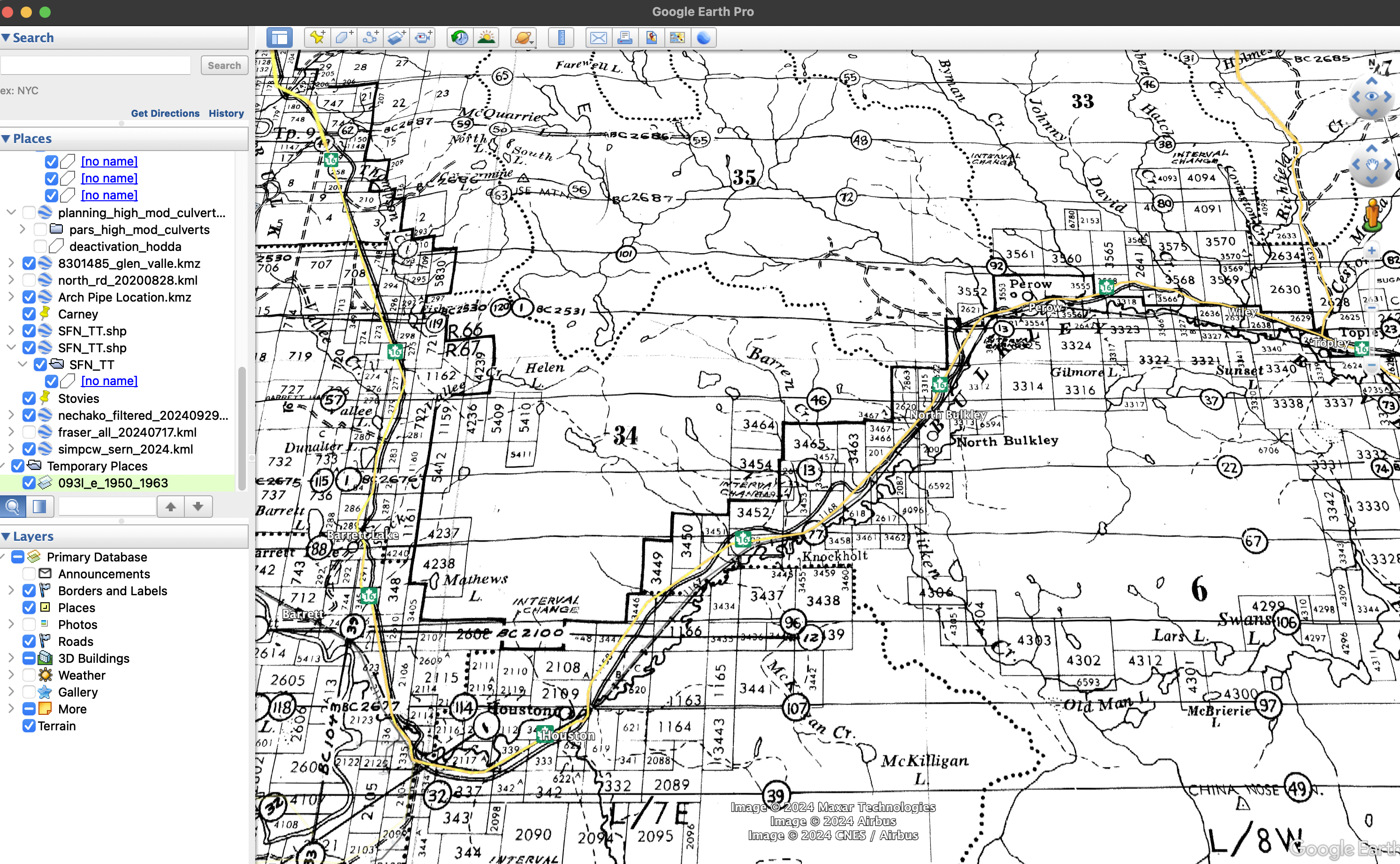
Figure 2: Screenshot of kml downloaded from link provided in Historic Imagery Points.

Historic Imagery Polygons

It appears we have the same sort of kml/pdf product as we saw in the Historic Imagery Points is being served through the Historic Imagery Polygons layer (Table 2).

Code

my_caption <- "The 'airborne-imagery-historical-index-map-points' datset for the area of interest"
#This what the information in the [Historic Imagery Points](https://catalogue.data.gov.bc.ca/dataset/airborne-imagery-historical-index-map-points) layer looks like.

layers_trimmed$l_imagery_hist_poly |> 
  dplyr::mutate(
    kml_url = ngr::ngr_str_link_url(
      url_base = "https://openmaps.gov.bc.ca/flight_indices/kml/large_scale", 
      url_resource = fs::path(basename(fs::path_dir(kml_url)), basename(kml_url))
    ),
    pdf_url = ngr::ngr_str_link_url(
      url_base = "https://openmaps.gov.bc.ca/flight_indices/pdf", 
      url_resource = fs::path(
        ngr::ngr_str_dir_from_path(pdf_url, levels = 3), 
        ngr::ngr_str_dir_from_path(pdf_url, levels = 2),
        ngr::ngr_str_dir_from_path(pdf_url, levels = 1),
        basename(pdf_url))
    )
  )|> 
  dplyr::select(-id) |> 
  sf::st_drop_geometry() |> 
  dplyr::arrange(start_year) |> 
  knitr::kable(
    escape = FALSE,
  caption = my_caption
  )

Table 2: The ‘airborne-imagery-historical-index-map-points’ datset for the area of interest

historical_index_map_id	scale_category	geoextent_mapsheet	map_tag	start_year	end_year	kml_url	pdf_url	feature_area_sqm	feature_length_m	objectid	se_anno_cad_data
866	medium	093l	093l_1	1938	1956	url_link	url_link	14421427749	481668.3	2183	NA
862	medium	093k	093k_2	1946	1956	url_link	url_link	14421427749	481668.3	2179	NA
557	large	093l_e	093l_e_1	1950	1963	url_link	url_link	7211433354	352456.5	1923	NA
549	large	093k_w	093k_w_1	1950	1963	url_link	url_link	7211433354	352456.5	1915	NA
863	medium	093k	093k_3	1961	1966	url_link	url_link	14421427749	481668.3	2180	NA
867	medium	093l	093l_2	1966	1972	url_link	url_link	14421427749	481668.3	2184	NA
550	large	093k_w	093k_w_2	1969	1973	url_link	url_link	7211433354	352456.5	1916	NA
1047	small	093nw	093nw_1	1970	1975	url_link	url_link	56959075420	956978.8	2312	NA
558	large	093l_e	093l_e_2	1971	1974	url_link	url_link	7211433354	352456.5	1924	NA
864	medium	093k	093k_4	1971	1971	url_link	url_link	14421427749	481668.3	2181	NA
559	large	093l_e	093l_e_3	1975	1975	url_link	url_link	7211433354	352456.5	1925	NA
551	large	093k_w	093k_w_3	1975	1980	url_link	url_link	7211433354	352456.5	1917	NA
865	medium	093k	093k_5	1977	1985	url_link	url_link	14421427749	481668.3	2182	NA
552	large	093k_w	093k_w_4	1978	1985	url_link	url_link	7211433354	352456.5	1918	NA
553	large	093k_w	093k_w_5	1978	1988	url_link	url_link	7211433354	352456.5	1919	NA
1048	small	093nw	093nw_2	1979	1979	url_link	url_link	56959075420	956978.8	2313	NA
560	large	093l_e	093l_e_4	1980	1980	url_link	url_link	7211433354	352456.5	1926	NA
561	large	093l_e	093l_e_5	1980	1980	url_link	url_link	7211433354	352456.5	1927	NA
562	large	093l_e	093l_e_6	1981	1983	url_link	url_link	7211433354	352456.5	1928	NA
868	medium	093l	093l_3	1981	1984	url_link	url_link	14421427749	481668.3	2185	NA
1049	small	093nw	093nw_3	1982	1984	url_link	url_link	56959075420	956978.8	2314	NA
554	large	093k_w	093k_w_6	1985	1988	url_link	url_link	7211433354	352456.5	1920	NA
1050	small	093nw	093nw_trim	1986	1988	url_link	url_link	64069901258	1020771.3	2315	NA
563	large	093l_e	093l_e_7	1989	1989	url_link	url_link	7211433354	352456.5	1929	NA
555	large	093k_w	093k_w_7	1989	1989	url_link	url_link	7211433354	352456.5	1921	NA
556	large	093k_w	093k_w_8	1990	1990	url_link	url_link	7211433354	352456.5	1922	NA
564	large	093l_e	093l_e_8	1990	1990	url_link	url_link	7211433354	352456.5	1930	NA

Air Photo Centroids

Each of the Air Photo Centroids are georeferenced with a date range of:

Code

range(layers_trimmed$l_photo_centroids$photo_date)

[1] "1963-08-07" "2019-09-18"

We visualize column metadata in Table 3 and map the centroids in our study area with Figure 3.

Code

# At this point we have downloaded two csvs (one for each NTS 1:50,000 mapsheet of course) with information about the airphotos including UTM coordinates that we will assume for now are the photo centres. In our next steps we read in what we have, turn into spatial object, trim to overall study area and plot.
# list csvs
ls <- fs::dir_ls(
  fs::path(
    path_post,
    "data"),
  glob = "*.csv"
)

photos_raw <- ls |> 
  purrr::map_df(
    readr::read_csv
  ) |> 
  sf::st_as_sf(
    coords = c("Longitude", "Latitude"), crs = 4326
  ) |> 
  janitor::clean_names() |> 
  dplyr::mutate(photo_date = lubridate::mdy(photo_date)) 


photos_aoi <- sf::st_intersection(
  photos_raw, 
  layers_trimmed$aoi |> st_make_valid()
  )

Code

bcdata::bcdc_describe_feature("WHSE_IMAGERY_AND_BASE_MAPS.AIMG_PHOTO_CENTROIDS_SP") |> 
  knitr::kable() |> 
  kableExtra::scroll_box(width = "100%", height = "500px")

Table 3: Metadata for the 'airphoto-centroids' layer in the BC Data Catalouge

col_name	sticky	remote_col_type	local_col_type	column_comments
id	TRUE	xsd:string	character	NA
AIRP_ID	TRUE	xsd:decimal	numeric	AIRP_ID is the unique photo frame identifier, generated by the source APS system.
FLYING_HEIGHT	FALSE	xsd:decimal	numeric	FLYING_HEIGHT is the flying height above mean sea level in metres.
PHOTO_YEAR	TRUE	xsd:decimal	numeric	PHOTO_YEAR is the operational year to which this photograph is assigned.
PHOTO_DATE	FALSE	xsd:date	date	PHOTO_DATE is the date (year, month, and day) of exposure of the photograph.
PHOTO_TIME	FALSE	xsd:string	character	PHOTO_TIME is the time of exposure (hours, minutes, seconds), expressed in Pacific Standard Time, e.g., 9:43:09 AM.
LATITUDE	FALSE	xsd:decimal	numeric	LATITUDE is the geographic coordinate, in decimal degrees (dd.dddddd), of the location of the feature as measured from the equator, e.g., 55.323653.
LONGITUDE	FALSE	xsd:decimal	numeric	LONGITUDE is the geographic coordinate, in decimal degrees (dd.dddddd), of the location of the feature as measured from the prime meridian, e.g., -123.093544.
FILM_ROLL	FALSE	xsd:string	character	FILM_ROLL is a BC Government film roll identifier, e.g., bc5624.
FRAME_NUMBER	FALSE	xsd:decimal	numeric	FRAME_NUMBER is the sequential frame number of this photograph within a film roll.
GEOREF_METADATA_IND	FALSE	xsd:string	character	GEOREF_METADATA_IND indicates if georeferencing metadata exists for this photograph, i.e., Y, N.
PUBLISHED_IND	FALSE	xsd:string	character	PUBLISHED_IND indicates if this photograph's geometry and metadata should be exposed for viewing, i.e., Y,N.
MEDIA	FALSE	xsd:string	character	MEDIA describes the photographic medium on which this photograph was recorded, e.g. Film - BW.
PHOTO_TAG	FALSE	xsd:string	character	PHOTO_TAG is a combination of film roll identifier and frame number that uniquely identifies an air photo, e.g., bcc09012_035.
BCGS_TILE	FALSE	xsd:string	character	BCGS_TILE identifies the BCGS mapsheet within which the centre of this photograph is contained. The BCGW mapsheet could be 1:20,000, 1:10,000 or 1:5,000, e.g., 104a01414.
NTS_TILE	FALSE	xsd:string	character	NTS_TILE identifies the NTS 1:50,000 mapsheet tile within which the centre of this photograph is contained, e.g., 104A03.
SCALE	FALSE	xsd:string	character	SCALE of the photo with respect to ground based on a 9-inch square hardcopy print, e.g., 1:18,000.
GROUND_SAMPLE_DISTANCE	FALSE	xsd:decimal	numeric	GROUND_SAMPLE_DISTANCE indicates the distance on the ground in centimetres represented by a single pixel in the scanned or original digital version of this photograph.
OPERATION_TAG	FALSE	xsd:string	character	OPERATION_TAG is an alpha numeric shorthand operation identifier representing photographic medium, operation number, requesting agency and operational year of photography, e.g., D003FI15.
FOCAL_LENGTH	FALSE	xsd:decimal	numeric	FOCAL_LENGTH is the focal length of the lens, in millimetres, used to capture this photograph.
THUMBNAIL_IMAGE_URL	FALSE	xsd:string	character	THUMBNAIL_IMAGE_URL is a hyperlink to the 1/16th resolution thumbnail version of this image.
FLIGHT_LOG_URL	FALSE	xsd:string	character	FLIGHT_LOG_URL is a hyperlink to the scanned version of the original handwritten flight log page (film record) for this image.
CAMERA_CALIBRATION_URL	FALSE	xsd:string	character	CAMERA_CALIBRATION_URL is a hyperlink to the camera calibration report file for this image.
PATB_GEOREF_URL	FALSE	xsd:string	character	PATB_GEOREF_URL is a hyperlink to the PatB geo-referencing file for this image.
FLIGHT_LINE_SEGMENT_ID	FALSE	xsd:decimal	numeric	FLIGHT_LINE_SEGMENT_ID identifies the section of flight line to which this photograph belongs.
OPERATION_ID	FALSE	xsd:decimal	numeric	OPERATION_ID is a unique identifier for the operation to which this photograph belongs. It may be used by the data custodian to diagnose positional errors.
FILM_RECORD_ID	FALSE	xsd:decimal	numeric	FILM_RECORD_ID is a unique identifier for the film record to which this photograph belongs. It may be used by the data custodian to diagnose positional errors.
SHAPE	FALSE	gml:PointPropertyType	sfc geometry	SHAPE is the column used to reference the spatial coordinates defining the feature.
OBJECTID	TRUE	xsd:decimal	numeric	OBJECTID is a column required by spatial layers that interact with ESRI ArcSDE. It is populated with unique values automatically by SDE.
SE_ANNO_CAD_DATA	FALSE	xsd:hexBinary	numeric	SE_ANNO_CAD_DATA is a binary column used by spatial tools to store annotation, curve features and CAD data when using the SDO_GEOMETRY storage data type.

Code

map +
  geom_sf(
    data = layers_trimmed$l_photo_centroids,
    alpha = 0.25
  )

Figure 3: ‘airphoto-centroids’ dataset for the area of interest.

That is a lot of photos! 9388 photos to be exact!!!

Refine Airphoto Centres by Clipping with Buffered Streams

Although we are likely moveing on to a different strategy - this section details how we can obtain imagery IDs for photo centres that fall within a pre-determined distance from streams of interest in our study area.

Code

# amount to buffer all stream segments
q_buffer <- 1500
# q_drm_main <- 263795

# length of streams other than selected explicity to buffer
q_drm_other <- 3000

Here are our query parameters to narrow down the area within our study are watershed in which we want to find photos for:

Buffer: 1500m - size of buffer used on either side of stream lines selected
Stream segments:
- Bulkley River (gnis_name in the stream layer)
- Maxan Creek
- Buck Creek
- for each remaining stream - segments of that stream which begin before 3000m from the downstream system (i.e. the first 3km) of stream.

Code

# We use the `downstream_route_measure` of the stream layer to exclude areas upstream of Bulkley Lake (also known as Taman Creek).  We find it in QGIS by highlighting the stream layer and clicking on our segment of interest while we have the information tool selected - the resulting pop-up looks like this in QGIS.
knitr::include_graphics(fs::path(
  path_post,
  "fig",
  "Screenshot2",
  ext = "png"
  )
)

Code

r_streams <- c("Maxan Creek", "Buck Creek")

aoi_refined_raw <- layers_trimmed$l_streams |> 
  # removed  & downstream_route_measure < q_drm_main for bulkley as doestn't cahnge 1960s query and increases beyond just by 5 photos
  dplyr::filter(gnis_name == "Bulkley River"|
                  gnis_name != "Bulkley River" & downstream_route_measure < q_drm_other |
                  gnis_name %in% r_streams) |> 
  # dplyr::arrange(downstream_route_measure) |>
  # calculate when we get to length_m by adding up the length_metre field and filtering out everything up to length_m
  # dplyr::filter(cumsum(length_metre) <= length_m) |>
  sf::st_union() |> 
  # we need to run st_sf or we get a sp object in a list...
  sf::st_sf()
  
aoi_refined_buffered <- sf::st_buffer(
  aoi_refined_raw,
  q_buffer, endCapStyle = "FLAT"
) 

photos_aoi_refined <- sf::st_intersection(
  layers_trimmed$l_photo_centroids, 
  aoi_refined_buffered
  )

Let’s plot again and include our buffered areas around the first 3000m of streams (area in red) along with the location of the photo points that land within that area. Looks like this give us 2770 photos.

Code

map +
  geom_sf(
    data = aoi_refined_buffered,
    color = "red",
    alpha= 0
  ) +
  geom_sf(
    data = photos_aoi_refined,
    alpha = 0.25,
  ) +
  geom_sf_text(
    data = layers_trimmed$l_streams |> dplyr::distinct(gnis_name, .keep_all = TRUE),
    aes(
      label = gnis_name
    ),
    size = 2  # Adjust size of the text labels as needed
  )

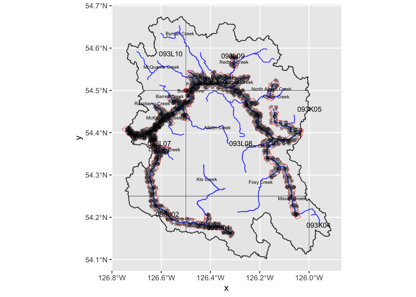
That is not as many photos - but still quite a few (2770).

Code

# @fig-dt1 below can be used to filter these photos from any time and/or mapsheet and export the result to csv or excel file.  
#| label: fig-dt1
#| tbl-cap: "All photo centroids located with watershed study area."
photos_aoi_refined |> 
  dplyr::select(-id) |> 
  my_dt_table(cols_freeze_left = 0)

Filter Photos by Date

Now lets map by year to see what our options are including the earliest photos possible. Here is our range to choose from:

Code

range(photos_aoi_refined$photo_date)

[1] "1963-08-07" "2019-09-18"

Code

map +
geom_sf(
  data = photos_aoi_refined |> dplyr::filter(photo_year <= "1975")
  ) +
  facet_wrap(~ photo_year)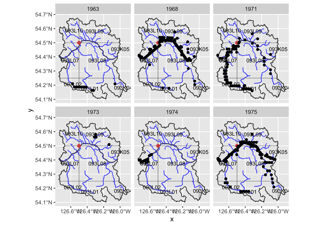

Well - looks like we get really good coverage of the Bulkley River mainstem in 1968 then much better coverage of the Buck Creek drainage and Maxan Creek in 1971. For 1975 - the coverage of the Bulkley mainstem and Maxan Creek is pretty good…

If we just wanted the areas near the river and we don’t mind mixing years - we grab the photos from:

1968 all
1971 for the Buck Creek and Maxan Creek areas only
1975 Maxan Creek only

Code

# spatially represent just Buck and Maxan, buffer and clip the 1971 photos
# "r_" is for "refine"
r_year1 <- "1968"
r_year2 <- "1971"
r_year3 <- "1975"

r_streams2 <- c("Maxan Creek")

l_streams_refined1 <- layers_trimmed$l_streams |> 
  # we defined r_streams in chunk way above 
  dplyr::filter(gnis_name %in% r_streams) |> 
  sf::st_union() |> 
  # we need to run st_sf or we get a sp object in a list...
  sf::st_sf()
  
aoi_refined_buffered2 <- sf::st_buffer(
  l_streams_refined1,
  q_buffer, endCapStyle = "FLAT"
) 

l_streams_refined2 <- layers_trimmed$l_streams |> 
  # we defined r_streams in chunk way above 
  dplyr::filter(gnis_name %in% r_streams2) |> 
  sf::st_union() |> 
  # we need to run st_sf or we get a sp object in a list...
  sf::st_sf()
  
aoi_refined_buffered3 <- sf::st_buffer(
  l_streams_refined2,
  q_buffer, endCapStyle = "FLAT"
) 

# filter first year
photos1 <- photos_aoi_refined |> 
  dplyr::filter(
      photo_year == r_year1
  )

# filter second year using just the streams we want to include
photos2 <- sf::st_intersection(
  layers_trimmed$l_photo_centroids |> dplyr::filter(photo_year == r_year2), 
  aoi_refined_buffered2
  )

# filter second year using just the streams we want to include
photos3 <- sf::st_intersection(
  layers_trimmed$l_photo_centroids |> dplyr::filter(photo_year == r_year3), 
  aoi_refined_buffered3
  )

photos_all <- dplyr::bind_rows(photos1, photos2, photos3)

Now let’s have a look at the individual year components (Figure 4) as well as the whole dataset (Figure 5). We are privileged to potentially have the assistance of Mike Price to help us obtain this imagery from the UBC archives. If there are too many photos to grab as is - the table below can be filtered by photo_year to reduce the number of photos. The resulting filtered dataset can then be downloaded by pressing the CSV or Excel buttons at the bottom of the table….

Code

my_caption <- "Amalgamated photo points presented by year."
map +
  geom_sf(
  data = photos_all
  ) +
  facet_wrap(~ photo_year)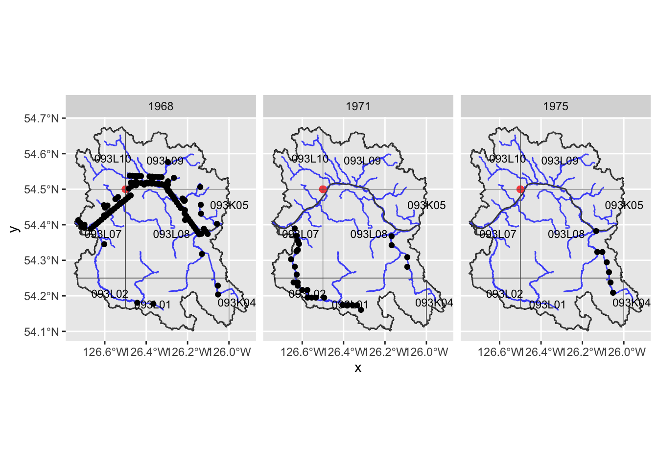

Figure 4: Amalgamated photo points presented by year.

Code

my_caption <- "Amalgamated photo points"
map +
  geom_sf(
  data = photos_all
  ) +
  geom_sf_text(
    data = layers_trimmed$l_streams |> dplyr::distinct(gnis_name, .keep_all = TRUE),
    aes(
      label = gnis_name
    ),
    size = 2  # Adjust size of the text labels as needed
  )

Export `csv` with Photo Information for Areas Adjacent to Streams

Let’s burn out a csv that can be used to find the imagery for the 253 photos above.

Code

lfile_name_photos <- function(dat = NULL){
  fs::path(
      path_post,
      "exports",
      paste(
        "airphotos",
        paste(range(dat$photo_date), collapse = "_"),
        sep = "_"
      ),
      ext = "csv"
    )
}

photos_all |> 
  readr::write_csv(
    lfile_name_photos(photos_all), na =""
  )


lpath_link <- function(dat = NULL){
  paste0(
    "https://github.com/NewGraphEnvironment/new_graphiti/tree/main/posts/2024-11-15-bcdata-ortho-historic/exports/",
    basename(
      lfile_name_photos(dat)
    )
  )
}

We can view and download exported csv files here but really we are perhaps better off using the widget below to get the csv file we need.

Code

photos_all |> 
  dplyr::select(-id) |> 
  my_dt_table(cols_freeze_left = 0)

Estimate Polygon Size based on the Scale and a 9” x 9” Negative

Here we take a shot at deriving the image footprint using the scale and a negative size of 9” X 9” which seems to be what is recorded in the flight logs (haven’t checked every single one yet).

Code

# not accurate!!!!!!!!!!!! this is for the equator!!!
# Add geometry
photos_poly_prep <- layers_trimmed$l_photo_centroids |> 
  dplyr::select(-id) |> 
  sf::st_drop_geometry() |> 
  # Parse scale
  dplyr::mutate(
    scale_parsed = as.numeric(stringr::str_remove(scale, "1:")),
    width_m = 9 * scale_parsed * 0.0254,  # Width in meters
    height_m = 9 * scale_parsed * 0.0254, # Height in meters
  ) |>
  # Create geometry
  dplyr::rowwise() |> 
  dplyr::mutate(
    geometry = list({
      # Create polygon corners
      center <- c(longitude, latitude)
      width_deg = (width_m / 2) / 111320  # Convert width to degrees (~111.32 km per degree latitude)
      height_deg = (height_m / 2) / 111320 # Approximate for longitude; accurate near equator
      
      # Define corners
      corners <- matrix(
        c(
          center[1] - width_deg, center[2] - height_deg, # Bottom-left
          center[1] + width_deg, center[2] - height_deg, # Bottom-right
          center[1] + width_deg, center[2] + height_deg, # Top-right
          center[1] - width_deg, center[2] + height_deg, # Top-left
          center[1] - width_deg, center[2] - height_deg  # Close the polygon
        ),
        ncol = 2,
        byrow = TRUE
      )
      
      # Create polygon geometry
      sf::st_polygon(list(corners))
    })
  ) |> 
  dplyr::ungroup() |>
  # Convert to sf object
  sf::st_as_sf(sf_column_name = "geometry", crs = 4326)

Code

photos_poly_prep <- layers_trimmed$l_photo_centroids |> 
  dplyr::select(-id) |> 
  sf::st_transform(crs = 32609) |>  # Transform to UTM Zone 9 for accurate metric calculations
  # Parse scale and calculate dimensions in meters
  dplyr::mutate(
    scale_parsed = as.numeric(stringr::str_remove(scale, "1:")),
    width_m = 9 * scale_parsed * 0.0254,  # Width in meters
    height_m = 9 * scale_parsed * 0.0254  # Height in meters
  ) |> 
  # Create geometry using UTM coordinates
  dplyr::rowwise() |> 
  dplyr::mutate(
    geometry = list({
      # Create polygon corners in UTM (meters)
      center <- sf::st_coordinates(geometry)  # Extract UTM coordinates
      width_half = width_m / 2
      height_half = height_m / 2
      
      # Define corners in meters
      corners <- matrix(
        c(
          center[1] - width_half, center[2] - height_half, # Bottom-left
          center[1] + width_half, center[2] - height_half, # Bottom-right
          center[1] + width_half, center[2] + height_half, # Top-right
          center[1] - width_half, center[2] + height_half, # Top-left
          center[1] - width_half, center[2] - height_half  # Close the polygon
        ),
        ncol = 2,
        byrow = TRUE
      )
      
      # Create polygon geometry
      sf::st_polygon(list(corners))
    })
  ) |> 
  dplyr::ungroup() |> 
  # Convert to sf object with UTM Zone 9 CRS
  sf::st_as_sf(sf_column_name = "geometry") |> 
  sf::st_set_crs(32609) |>  # Assign UTM Zone 9 CRS
  # Transform back to WGS84 (if needed)
  sf::st_transform(crs = 4326)

Code

# Assuming `photos_poly` has a `photo_year` column with years of interest
photos_poly <- photos_poly_prep |> 
  dplyr::filter(
    photo_year %in% c(1968, 1971, 1975)
    )

l_photo_centroids_fltered <- layers_trimmed$l_photo_centroids |> 
      dplyr::filter(
        photo_year %in% c(1968, 1971, 1975)
    )

years <- unique(photos_poly$photo_year)

years_centroids <- unique(l_photo_centroids_fltered$photo_year)

map <- my_leaflet()

# Loop through each year and add polygons with the year as a group
for (year in years) {
  map <- map |> 
    leaflet::addPolygons(
      data = photos_poly |> 
        dplyr::filter(
          photo_year == year
          ), 
      color = "black", 
      weight = 1, 
      smoothFactor = 0.5,
      opacity = 1.0, 
      fillOpacity = 0,
      group = paste0("Polygons - ", year)
    )
}

# Add centroid layers for each year
for (year in years_centroids) {
  map <- map |> 
    leaflet::addCircleMarkers(
      data = l_photo_centroids_fltered |> dplyr::filter(photo_year == year),
      radius = 1,
      color = "black",
      fillOpacity = 0.7,
      opacity = 1.0,
      group = paste0("Centroids - ", year)
    )
}

all_groups <- c(paste0("Polygons - ", years), paste0("Centroids - ", years_centroids))

# Add layer control to toggle year groups
map <- map |> 
  leaflet::addPolygons(
    data = layers_trimmed$aoi, 
              color = "black", 
              weight = 1, 
              smoothFactor = 0.5,
              opacity = 1.0, 
              fillOpacity = 0
              ) |> 
  # leaflet::addPolygons(
  #   data = layers_trimmed$aoi_raw, 
  #             color = "yellow", 
  #             weight = 1, 
  #             smoothFactor = 0.5,
  #             opacity = 1.0, 
  #             fillOpacity = 0
  #             ) |> 
  leaflet::addLayersControl(
    baseGroups = c(
      "Esri.DeLorme",
      "ESRI Aerial"),
    overlayGroups = all_groups,
    options = leaflet::layersControlOptions(collapsed = FALSE)
  ) |> 
  leaflet.extras::addFullscreenControl()

map

Figure 6

Build a Interactive Dashboard that allows us to Visualize and Download by a Specific Year

Use the filter and slider to see the coverage for photos we have for an individual year then export to excel or csv file with the buttons at the bottom of the table below.

Code

# Wrap data frame in SharedData
sd <- crosstalk::SharedData$new(
  layers_trimmed$l_photo_centroids |> 
    dplyr::mutate(
      thumbnail_image_url = ngr::ngr_str_link_url(
        url_base = "https://openmaps.gov.bc.ca/thumbs", 
        url_resource = 
          fs::path_rel(
            thumbnail_image_url, start = "https://openmaps.gov.bc.ca/thumbs"
          )
      ),
      flight_log_url = ngr::ngr_str_link_url(
        url_base = "https://openmaps.gov.bc.ca/thumbs/logbooks/", 
        url_resource = 
          fs::path_rel(flight_log_url, start = "https://openmaps.gov.bc.ca/thumbs/logbooks/")
      )
    )|> 
    
    dplyr::select(-id)
)


# Use SharedData like a dataframe with Crosstalk-enabled widgets
map3 <- sd |>
  leaflet::leaflet(height = 500) |> #height=500, width=780
  leaflet::addProviderTiles("Esri.WorldTopoMap", group = "Topo") |>
  leaflet::addProviderTiles("Esri.WorldImagery", group = "ESRI Aerial") |>
  leaflet::addCircleMarkers(
    radius = 3,
    fillColor = "black",
    color= "#ffffff",
    stroke = TRUE,
    fillOpacity = 1.0,
    weight = 2,
    opacity = 1.0
  ) |>
  leaflet::addPolylines(data=layers_trimmed$l_streams,
               opacity=0.75, 
               color = 'blue',
               fillOpacity = 0.75, 
               weight=2) |> 
    leaflet::addPolygons(
    data = layers_trimmed$aoi, 
              color = "black", 
              weight = 1, 
              smoothFactor = 0.5,
              opacity = 1.0, 
              fillOpacity = 0
              ) |> 
  leaflet::addLayersControl(
    baseGroups = c(
      "Esri.DeLorme",
      "ESRI Aerial"),
    options = leaflet::layersControlOptions(collapsed = F)) |> 
  leaflet.extras::addFullscreenControl(position = "bottomright") |> 
  leaflet::addScaleBar(position = "bottomleft")


widgets <- crosstalk::bscols(
  widths = c(3, 9),
  crosstalk::filter_checkbox(
    id = "label",
    label =  "Media Type",
    sharedData = sd,
    group =  ~media
  ),
  crosstalk::filter_slider(
    id = "year_slider",
    label = "Year",
    sharedData = sd,
    column = ~photo_year,
    round = 0
  )
)

htmltools::browsable(
  htmltools::tagList(
    widgets,
    map3,
    sd |> my_dt_table(page_length = 5, escape = FALSE)
  )
)

Media Type

Digital - Colour

Film - BW

Film - Colour

Year

How many different flight log records are there?

What are the unique values of scale reported?

1:10000, 1:12000, 1:15000, 1:15840, 1:16000, 1:18000, 1:20000, 1:30000, 1:31680, 1:40000, 1:50000, 1:60000, 1:70000, 1:8000, 9600

Thinkgs to do

According to Figure 2 some images have been georeferenced. However, using a kml with basically a picture drawn on it showing what appears to be the airp_id seems like a very difficult task. Guessing there is a decent chance that there is a digital file somewhere within the gov that details which airp_ids are on which kml/pdf and we could use that to remove photos from our chosen year from ones we wish to aquire and georeference.

Generate an Area of Interest

Download Spatial Data Layers From BC DAta Catalogue

Map the Area of Interest

Explore the BC Data Catalouge Imagery Layer Options

Orthophoto Tile Polygons

Historic Imagery Points

Historic Imagery Polygons

Air Photo Centroids

Refine Airphoto Centres by Clipping with Buffered Streams

Filter Photos by Date

Export csv with Photo Information for Areas Adjacent to Streams

Estimate Polygon Size based on the Scale and a 9” x 9” Negative

Build a Interactive Dashboard that allows us to Visualize and Download by a Specific Year

Thinkgs to do

Export `csv` with Photo Information for Areas Adjacent to Streams