2 Explore FWA Streams

Purpose of this section was to explore the lengths and frequencies of double lined streams as there is a channel width predictor model channel-width-21. Result of this work was that Simon has sampled each double line stream 30 times and kept the average and standard deviation - regarless of segment length bcfishpass.

Load the double line streams used in channel_width_mapped. In order to facilitate reproducability lets save the streams in a sqlite and pull them back in.

##gconnect to database
conn <- DBI::dbConnect(
  RPostgres::Postgres(),
  dbname = dbname_wsl,
  host = host_wsl,
  port = port_wsl,
  user = user_wsl,
  password = password_wsl
)



##get the segments that have a centreline (double line streams)
q <- ("SELECT linear_feature_id, ceil(upstream_route_measure)::integer - floor(downstream_route_measure)::integer AS len,
      watershed_group_code
      FROM whse_basemapping.fwa_stream_networks_sp 
      WHERE edge_type = 1250")

streams <- sf::st_read(conn, query = q) 



##  the streams in a sqlite and pull them back in.
##########################!!!!!!!!!!!!!!!!!!!!!!!!!!!!!!!!!!!#########################
###change this up so that it matches your version of the ahred dropbox!




mydb <- DBI::dbConnect(RSQLite::SQLite(), paste0(shared_dropbox_dir, "fiss/fissr_explore.sqlite"))


conn <- readwritesqlite::rws_connect(paste0(shared_dropbox_dir, "fiss/fissr_explore.sqlite"))
readwritesqlite::rws_write(streams, exists = F, delete = TRUE,
          conn = conn, x_name = "whse_basemapping.fwa_stream_networks_sp")
readwritesqlite::rws_list_tables(conn)
readwritesqlite::rws_disconnect(conn)

shared_dropbox_dir <- "C:/Users/al/Dropbox/New Graph/"

Load the streams from sqlite. The table I pull back in after saving as sqlite has linear_feature_id as integer vs int64 as it was pulled from postgres. No issues for this exercise though…

conn <- readwritesqlite::rws_connect(paste0(shared_dropbox_dir, "fiss/fissr_explore.sqlite"))
streams <- readwritesqlite::rws_read_table("whse_basemapping.fwa_stream_networks_sp", conn = conn)
readwritesqlite::rws_disconnect(conn)

summary(streams$len)

##    Min. 1st Qu.  Median    Mean 3rd Qu.    Max. 
##     1.0    86.0   181.0   294.5   362.0  9253.0

Lets look at distribution of lengths

ggplot(select(streams, len), aes(x=len)) +
  geom_histogram(position="identity", size = 0.75)+
  labs(x = "length", y = "#") +
  ggdark::dark_theme_bw(base_size = 11)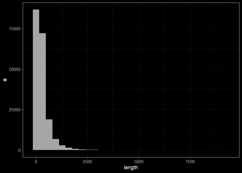

##segments less than 1000m long
ggplot(select(streams, len) %>% filter(len < 1000), aes(x=len)) +
  geom_histogram(position="identity", size = 0.75)+
  labs(x = "length", y = "#") +
  ggdark::dark_theme_bw(base_size = 11)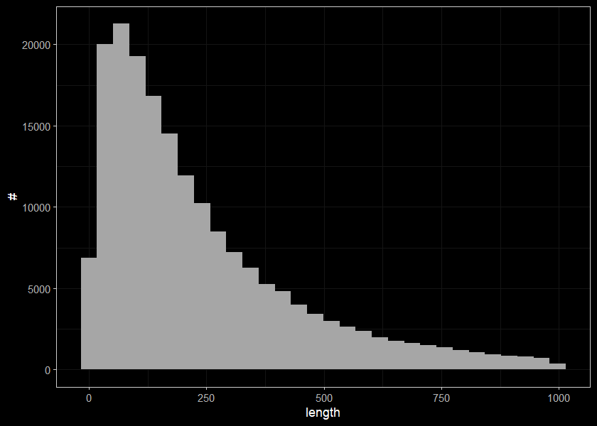

##segments less than 250m long
ggplot(select(streams, len) %>% filter(len < 250), aes(x=len)) +
  geom_histogram(position="identity", size = 0.75)+
  labs(x = "length", y = "#") +
  ggdark::dark_theme_bw(base_size = 11)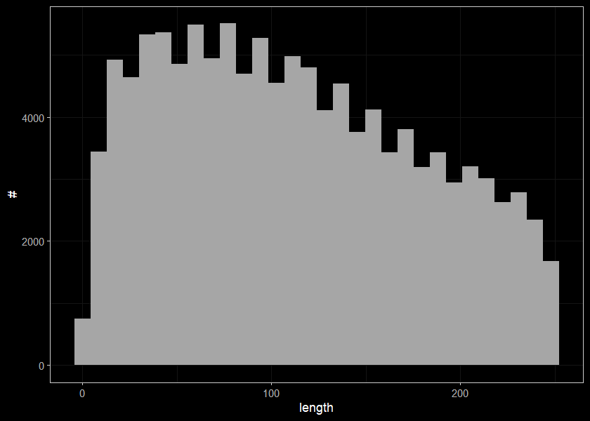

##how many streams are segments are smaller than 50m
streams %>% 
  filter(len > 1000) %>% 
  count()

## # A tibble: 1 x 1
##       n
##   <int>
## 1  8286

streams_equal <- streams %>% 
  mutate(cut = cut_number(len, n = 5)) %>% 
  group_by(cut) %>% 
  summarise(n = n())

streams_equal

## # A tibble: 5 x 2
##   cut                n
##   <fct>          <int>
## 1 [1,70]         38500
## 2 (70,138]       38232
## 3 (138,235]      37768
## 4 (235,427]      38064
## 5 (427,9.25e+03] 38099

streams_interval <- streams %>% 
  mutate(cut = cut_interval(len, n = 10)) %>% 
  group_by(cut) %>% 
  summarise(n = n())

streams_interval

## # A tibble: 10 x 2
##    cut                      n
##    <fct>                <int>
##  1 [1,926]             180821
##  2 (926,1.85e+03]        8096
##  3 (1.85e+03,2.78e+03]   1296
##  4 (2.78e+03,3.7e+03]     294
##  5 (3.7e+03,4.63e+03]      90
##  6 (4.63e+03,5.55e+03]     33
##  7 (5.55e+03,6.48e+03]     21
##  8 (6.48e+03,7.4e+03]       7
##  9 (7.4e+03,8.33e+03]       4
## 10 (8.33e+03,9.25e+03]      1

streams_length <- streams %>%
  mutate(cut =
           case_when(
             len < 100 ~ '0_100',
             len >= 100 & len < 500 ~ '0100_500',
             len >= 500 & len < 999 ~ '0500_1000',
             len >=999  ~ '1000+')) 

streams_length_sum <- streams_length %>% 
  group_by(cut) %>% 
  summarise(n = n())

streams_length_sum

## # A tibble: 4 x 2
##   cut            n
##   <chr>      <int>
## 1 0_100      55821
## 2 0100_500  104540
## 3 0500_1000  21988
## 4 1000+       8314

ggplot(data = streams_length_sum, mapping = aes(x=cut, y = n)) + 
  geom_bar(stat = "identity") + 
  # ylim(1000, 20000)+
  # labs(x='test') +
  ggdark::dark_theme_bw(base_size = 11)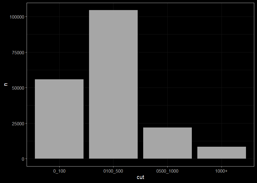

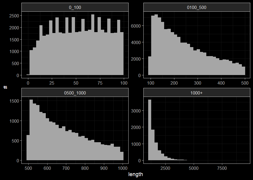
ggplot(streams_length, aes(x=len)) +
  geom_histogram(position="identity", size = 0.75)+
  labs(x = "length", y = "#") +
  facet_wrap(~cut, ncol = 2, scales = "free")+
  ggdark::dark_theme_bw(base_size = 11)