3 Results and Discussion
Results of Phase 1 and Phase 2 assessments are summarized in Figure 3.1 with additional details provided in sections below.
##make colors for the priorities
pal <-
   colorFactor(palette = c("red", "yellow", "grey", "black"),
               levels = c("high", "moderate", "low", "no fix"))

pal_phase1 <-
   colorFactor(palette = c("red", "yellow", "grey", "black"),
               levels = c("high", "moderate", "low", NA))

# tab_map_phase2 <- tab_map %>% filter(source %like% 'phase2')
#https://stackoverflow.com/questions/61026700/bring-a-group-of-markers-to-front-in-leaflet
# marker_options <- markerOptions(
#   zIndexOffset = 1000)
tracks <- sf::read_sf("./data/habitat_confirmation_tracks.gpx", layer = "tracks")


wshd_study_areas <- sf::read_sf('data/fishpass_mapping/wshd_study_areas.geojson')
  # st_transform(crs = 4326)

map_phase3 <- bcfishpass %>%
  filter(aggregated_crossings_id %in% c(125179, 125000, 125261, 125231, 1016602819)) %>%
  mutate(stream_crossing_id = case_when(aggregated_crossings_id == 1016602819 ~ 125345,
                                        T ~ stream_crossing_id)) %>%
    sf::st_as_sf(coords = c("utm_easting", "utm_northing"),
               crs = 26910, remove = F) %>% ##don't forget to put it in the right crs buds
  sf::st_transform(crs = 4326)

map_phase4 <- map_phase3 %>%
  filter(stream_crossing_id == 125179)

map <- leaflet(height=500, width=780) %>%
  addTiles()  %>%
  # leafem::addMouseCoordinates(proj4 = 26911) %>% ##can't seem to get it to render utms yet
  # addProviderTiles(providers$"Esri.DeLorme") %>%
  addProviderTiles("Esri.WorldTopoMap", group = "Topo") %>%
  addProviderTiles("Esri.WorldImagery", group = "ESRI Aerial") %>%
  addPolygons(data = wshd_study_areas, color = "#F29A6E", weight = 1, smoothFactor = 0.5,
              opacity = 1.0, fillOpacity = 0,
              fillColor = "#F29A6E", label = wshd_study_areas$watershed_group_name) %>%

  addPolygons(data = wshds, color = "#0859C6", weight = 1, smoothFactor = 0.5,
              opacity = 1.0, fillOpacity = 0.25,
              fillColor = "#00DBFF",
              label = wshds$stream_crossing_id,
              popup = leafpop::popupTable(x = select(wshds %>% st_set_geometry(NULL),
                                                     Site = stream_crossing_id,
                                                     elev_min:area_km),
                                          feature.id = F,
                                          row.numbers = F),
              group = "Confirmation 2022") %>%
  addLegend(
    position = "topright",
    colors = c("red", "yellow", "grey", "black"),
    labels = c("High", "Moderate", "Low", 'No fix'), opacity = 1,
    title = "Fish Passage Priorities") %>%
#   # addCircleMarkers(
#   # data=tab_plan_sf,
#   # label = tab_plan_sf$Comments,
#   # labelOptions = labelOptions(noHide = F, textOnly = F),
#   # popup = leafpop::popupTable(x = tab_plan_sf %>% st_drop_geometry(),
#   #                             feature.id = F,
#   #                             row.numbers = F),
#   # radius = 9,
#   # fillColor = ~pal_phase1(tab_plan_sf$Priority),
#   # color= "#ffffff",
#   # stroke = TRUE,
#   # fillOpacity = 1.0,
# # weight = 2,
# # opacity = 1.0,
# # group = "Planning") %>%
addCircleMarkers(data=tab_map %>%
                   filter(source %like% 'phase1' | source %like% 'pscis_reassessments'),
                 label = tab_map %>% filter(source %like% 'phase1' | source %like% 'pscis_reassessments') %>% pull(pscis_crossing_id),
                 # label = tab_map$pscis_crossing_id,
                 labelOptions = labelOptions(noHide = F, textOnly = TRUE),
                 popup = leafpop::popupTable(x = select((tab_map %>% st_set_geometry(NULL) %>% filter(source %like% 'phase1' | source %like% 'pscis_reassessments')),
                                                        Site = pscis_crossing_id, Priority = priority_phase1, Stream = stream_name, Road = road_name, `Habitat value`= habitat_value, `Barrier Result` = barrier_result, `Culvert data` = data_link, `Culvert photos` = photo_link, `Model data` = model_link),
                                             feature.id = F,
                                             row.numbers = F),
                 radius = 9,
                 fillColor = ~pal_phase1(priority_phase1),
                 color= "#ffffff",
                 stroke = TRUE,
                 fillOpacity = 1.0,
                 weight = 2,
                 opacity = 1.0,
                 group = "Assessment 2022") %>%
  addPolylines(data=tracks,
               opacity=0.75, color = '#e216c4',
               fillOpacity = 0.75, weight=5, group = "Confirmation 2022") %>%

addAwesomeMarkers(
    lng = as.numeric(photo_metadata$gps_longitude),
    lat = as.numeric(photo_metadata$gps_latitude),
    popup = leafpop::popupImage(photo_metadata$url, src = "remote"),
    clusterOptions = markerClusterOptions(),
    group = "Confirmation 2022") %>%

  addCircleMarkers(
    data=tab_hab_map,
    label = tab_hab_map$pscis_crossing_id,
    labelOptions = labelOptions(noHide = T, textOnly = TRUE),
    popup = leafpop::popupTable(x = select((tab_hab_map %>% st_drop_geometry()),
                                           Site = pscis_crossing_id,
                                           Priority = priority,
                                           Stream = stream_name,
                                           Road = road_name,
                                           `Habitat (m)`= upstream_habitat_length_m,
                                           Comments = comments,
                                           `Culvert data` = data_link,
                                           `Culvert photos` = photo_link,
                                           `Model data` = model_link),
                                feature.id = F,
                                row.numbers = F),
    radius = 9,
    fillColor = ~pal(priority),
    color= "#ffffff",
    stroke = TRUE,
    fillOpacity = 1.0,
    weight = 2,
    opacity = 1.0,
    group = "Confirmation 2022"
    ) %>%

    addCircleMarkers(
    data=map_phase3,
    label = map_phase3$stream_crossing_id,
    labelOptions = labelOptions(noHide = T, textOnly = TRUE),
    popup = leafpop::popupTable(x = select((map_phase3 %>% st_drop_geometry()),
                                           Site = stream_crossing_id,
                                           Stream = pscis_stream_name,
                                           Road = pscis_road_name,
                                           Comments = pscis_assessment_comment),
                                feature.id = F,
                                row.numbers = F),
    radius = 9,
    fillColor = "red",
    color= "#ffffff",
    stroke = TRUE,
    fillOpacity = 1.0,
    weight = 2,
    opacity = 1.0,
    group = "Design"
    ) %>%

      addCircleMarkers(
    data=map_phase4,
    label = map_phase4$stream_crossing_id,
    labelOptions = labelOptions(noHide = T, textOnly = TRUE),
    popup = leafpop::popupTable(x = select((map_phase3 %>% st_drop_geometry()),
                                           Site = stream_crossing_id,
                                           Stream = pscis_stream_name,
                                           Road = pscis_road_name,
                                           Comments = pscis_assessment_comment),
                                feature.id = F,
                                row.numbers = F),
    radius = 9,
    fillColor = "red",
    color= "#ffffff",
    stroke = TRUE,
    fillOpacity = 1.0,
    weight = 2,
    opacity = 1.0,
    group = "Remediation"
    ) %>%

  addLayersControl(
    baseGroups = c(
      "Esri.DeLorme",
      "ESRI Aerial"),
    overlayGroups = c("Assessment 2022", "Confirmation 2022", "Design", "Remediation"),
    options = layersControlOptions(collapsed = F)) %>%
  leaflet.extras::addFullscreenControl() %>%
  addMiniMap(tiles = providers$"Esri.NatGeoWorldMap",
             zoomLevelOffset = -6, width = 100, height = 100)

map %>%
  hideGroup(c("Assessment 2022", "Confirmation 2022"))
Figure 3.1: Map of target sites. Full screen available through button below zoom.
Identify and Communicate Connectivity Issues
Engage Partners
SERNbc and McLeod Lake have been actively engaging with the following groups to build awareness for the initiative, solicit input, prioritize sites, raise partnership funding and plan/implement fish passage remediations:
- McLeod Lake Indian Band members of council
- BCTS Engineering
- CN Rail
- Canadian Forest Products (Canfor)
- Sinclar Forest Projects Ltd. (Sinclar)
- Northern Engineering - Ministry of Forests
- BC Ministry of Transportation and Infrastructure
- Fish Passage Technical Working Group
- Coastal Gasliink
- British Columbia Wildlife Federation
- Planning foresters and biologists Ministry of Forests, Lands, Natural Resource Operations and Rural Development (restructured into Ministry of Forests and Ministry of Land, Water and Resource Stewardship)
- Fisheries experts
The Environmental Stewardship Initiative (ESI) is a collaborative partnership between the Province and First Nations with projects designed to focus on ecosystem assessment, restoration, enhancement, research and education. To date, four regional environmental stewardship projects have been developed throughout northern British Columbia. A governance working group with representatives from all four stewardship forums provides governance oversight and guidance for the ESI. The Parsnip River watershed group is within the Regional Strategic Environmental Assessment Forum (RSEA) area. Indigenous partners for RSEA include McLeod lake, Blueberry River, Halfway River, Doig River, West Moberly, Prophet River and Sauteau. Forum values of focus to date include old forest/forest biodiversity, water, moose, peaceful enjoyment and environmental livelihoods. Working together with McLeod Lake Indian Band we are leveraging RSEA initiatives by overlaying Parsnip River watershed group fish passage planning data with the Recreational Opportunity Spectrum Inventory data to facilitate discussions with partners and stakeholders about how long term landscape stewardship goals of McLeod Lake Indian Band relate to stream crossing infrastructure upgrades/removals within their traditional territory. The inventory data summarizes recreation opportunities as combinations of settings and probable human experience opportunities organized along a spectrum of classes. The spectrum is set out in terms of seven classes as follows: Primitive (P), Semi-primitive Non-motorized (SPNM), Semi-primitive Motorized (SPM), Roaded Natural (RN), Roaded Modified (RM), Rural (R), Urban (U). Areas classified towards the primitive end of the spectrum provide more opportunities for First Nations groups such as the McLeod Lake Indian Band to exercise their rights as indigenous people in areas less disturbed by industrial activity within their traditional territory (United Nations General Assembly 2007).
Mapping
Georeferenced field maps containing updated modelling outputs are presented in here and available for bulk download as Attachment 1.
Interactive Dashboard
The interactive dashboard is presented in Figure 3.2.
# join bcfishpass to some pscis columns for the screening table
# get our dataframe to link to a map
# xings filtered by >1km of potential rearing habitat
xf <- left_join(
  bcfishpass %>%
    st_as_sf(coords = c('utm_easting', 'utm_northing'), crs = 26910, remove = F) %>%
    filter(is.na(pscis_status) | (pscis_status != 'HABITAT CONFIRMATION' &
                                    barrier_status != 'PASSABLE' &
                                    barrier_status != 'UNKNOWN')) %>%
    filter(bt_rearing_km > 0.499) %>%
    filter(crossing_type_code != 'OBS') %>%
    filter(is.na(barriers_anthropogenic_dnstr)) %>%
    # rename(bt_rearing_km_raw = bt_rearing_km) %>%
    # mutate(bt_rearing_km = case_when(
    #   bt_rearing_km_raw >= 1 & bt_rearing_km_raw < 2 ~ '1-2km',
    #   bt_rearing_km_raw >= 2 & bt_rearing_km_raw <= 5 ~ '2-5km',
    #   bt_rearing_km_raw >= 5 & bt_rearing_km_raw <= 10 ~ '5-10km',
    #   T ~ '>10km')
    # ) %>%
    # mutate(bt_rearing_km = factor(bt_rearing_km, levels = c('1-2km', '2-5km', '5-10km', '>10km'))) %>%
    select(id = aggregated_crossings_id,
           pscis_status,
           barrier_status,
           contains('bt_'),
           utm_easting,
           utm_northing,
           gradient_gis = gradient,
           mapsheet = dbm_mof_50k_grid,
           watershed_group_code) %>%
    # need to run rowise for our fpr function to hit each row
    mutate(map_link = paste0('https://hillcrestgeo.ca/outgoing/fishpassage/projects/parsnip/archive/2022-05-27/FishPassage_', mapsheet, '.pdf')) %>%
    mutate(map_link = paste0("<a href ='", map_link,"'target='_blank'>", map_link,"</a>")) %>%
    arrange(id) %>%
    st_transform(crs = 4326),

  pscis %>%
    mutate(stream_crossing_id = as.character(stream_crossing_id)) %>%
    select(
      stream_crossing_id,
      stream_name,
      road_name,
      outlet_drop,
      channel_width = downstream_channel_width,
      habitat_value_code,
      image_view_url,
      assessment_comment) %>%
    mutate(image_view_url = paste0("<a href ='", image_view_url,"'target='_blank'>",image_view_url,"</a>")) %>%
    st_drop_geometry(),

  by = c('id' = 'stream_crossing_id')) %>%
  select(id,
         stream_name,
         habitat_value = habitat_value_code,
         mapsheet,
         map_link,
         image_view_url,
         pscis_status:bt_slopeclass15_km,
         bt_spawning_km:gradient_gis,
         # bt_spawning_km,
         # bt_rearing_km_raw:gradient_gis,
         road_name:assessment_comment,
         watershed_group_code)
  # dplyr::relocate(assessment_comment, .after = last_col())


# xf %>%
#   filter(!is.na(pscis_status))
#
# t <- xf %>%
#   group_by(bt_rearing_km) %>%
#   summarise(n = n())
# Wrap data frame in SharedData
sd <- SharedData$new(xf %>% select(-mapsheet))
# Use SharedData like a dataframe with Crosstalk-enabled widgets
map <- sd %>%
leaflet(height=500) %>% #height=500, width=780
# addTiles() %>%
addProviderTiles("Esri.WorldTopoMap", group = "Topo") %>%
addProviderTiles("Esri.WorldImagery", group = "ESRI Aerial") %>%
addCircleMarkers(
label = xf$id,
labelOptions = labelOptions(noHide = T, textOnly = TRUE),
popup = leafpop::popupTable(xf %>%
st_drop_geometry() %>%
select(id,
stream_name,
bt_rearing_km,
# bt_rearing_km = bt_rearing_km_raw,
bt_spawning_km,
mapsheet,
image_view_url,
assessment_comment,
watershed_group_code),
feature.id = F,
row.numbers = F),
radius = 9,
fillColor = "red",
color= "#ffffff",
stroke = TRUE,
fillOpacity = 1.0,
weight = 2,
opacity = 1.0
) %>%
addPolygons(data = wshd_study_areas, color = "#F29A6E", weight = 1, smoothFactor = 0.5,
opacity = 1.0, fillOpacity = 0,
fillColor = "#F29A6E", label = wshd_study_areas$watershed_group_name) %>%
addLayersControl(
baseGroups = c(
"Esri.DeLorme",
"ESRI Aerial"),
options = layersControlOptions(collapsed = F)) %>%
leaflet.extras::addFullscreenControl(position = "bottomright")
# tbl <- reactable::reactable(
# sd,
# selection = "multiple",
# onClick = "select",
# rowStyle = list(cursor = "pointer"),
# defaultPageSize = 5
# # minRows = 10
# )
# htmltools::browsable(
# htmltools::tagList(map, tbl)
# )
widgets <- bscols(
widths = c(2, 5, 5),
filter_checkbox("label",
"Watershed Group",
sd,
~watershed_group_code),
filter_slider(id = "label",
label = "Bull Trout Rearing (km)",
sharedData = sd,
column = ~bt_rearing_km,
round = 1,
min = 0,
max = 100),
filter_slider(id = "label",
label = "Bull Trout Spawning (km)",
sharedData = sd,
column = ~bt_spawning_km,
round = 1,
max = 45)
)
htmltools::browsable(
htmltools::tagList(
widgets,
map,
datatable(sd,
class = 'cell-border stripe',
extensions=c("Scroller","Buttons","FixedColumns"),
style="bootstrap",
# class="compact",
width="100%",
rownames = F,
options=list(
deferRender=TRUE,
scrollY=300,
scrollX = T,
scroller=TRUE,
dom = 'Bfrtip',
buttons = list(
'copy',
list(
extend = 'collection',
buttons = c('csv'),
text = 'Download csv')),
fixedColumns = list(leftColumns = 2),
initComplete = JS("function(settings, json) {","$(this.api().table().container()).css({'font-size': '11px'});","}")),
escape = F)
))my_photo = 'fig/pixel.png'
my_caption= 'Dashboard to facilitate field planning for field surveys. Note that only sites modelled with no crossings and having 0.5km or more of bull trout rearing habitat (>1.5m channel width and <7.5% gradient). Full screen available through button in bottom right of map.'
knitr::include_graphics(my_photo, dpi = NA)Figure 3.2: Dashboard to facilitate field planning for field surveys. Note that only sites modelled with no crossings and having 0.5km or more of bull trout rearing habitat (>1.5m channel width and <7.5% gradient). Full screen available through button in bottom right of map.
# identical(gitbook_on, FALSE)
my_caption = 'Field planning results to facilitate selection of restoration opportunities for 2022 field surveys.'

xf %>%
  sf::st_drop_geometry() %>%
  select(id:habitat_value,
         outlet_drop,
         bt_spawning_km,
         bt_rearing_km,
         mapsheet,
         utm_easting,
         utm_northing,
         assessment_comment) %>%

  # test by removing the html
  select(-mapsheet) %>%
  fpr::fpr_kable(caption_text = my_caption,
                 scroll = gitbook_on)
  # fpr_kable(caption_text = caption_text,
  #           scroll = gitbook_on)
Remediations
Tributary to Missinka River - PSCIS crossing 125179
PSCIS crossing 125179 is located on a tributary to Missinka River, 1km upstream of the confluence, on the Chuchinka-Missinka FSR. This crossing is located approximately 660m east of PSCIS crossing 125180 and joins this adjacent stream just before emptying into the Missinka River. A map of the watershed is provided in map attachment 93I.116. The twin culverts were replaced with a clear-span bridge in the summer of 2022.
In 2018, the Missinka River watershed was designated as a fisheries sensitive watershed under the authority of the Forest and Range Practices Act due to significant downstream fisheries values and watershed sensitivity (Beaudry 2013). Special management is required in the crossing’s watershed to protect habitat for Bull Trout and Arctic Grayling and includes measures (among others) to limit equivalent clearcut area, reduce impacts to natural stream channel morphology, retain old growth attributes and maintain fish habitat/movement.
The site was first assessed by A. Irvine (2020) in 2019 with reporting available here. At that time, there were two 1.2m diameter culverts side by side. The crossing was ranked as a high priority for follow up due to the 2km of suitable upstream high value habitat, where the presence of bull trout and rainbow trout had been previously confirmed. In 2020, with support from FWCP funding, an engineering design was commissioned for the site with funding acquired from the Ministry of Forests, Lands and Natural Resource Development in 2020 for project materials (riprap and girders). In the summer of 2022, a 15m steel girder permanent bridge with modular timber decks was installed. Crews visited the site in August of 2022. Photos showing a comparison of the culvert assessment conducted in 2019 versus the completed bridge construction in 2022 are presented in Figures 3.3 - 3.4. During the site visit aerial imagery was collected with a remotely piloted aircraft with resulting images stitched into an orthomosaic and 3-dimensional model presented in Figures 3.5 - 3.6. Bridge construction details including as-built drawings have been loaded to the PSCIS data portal for upload to the province.
my_photo1 = fpr::fpr_photo_pull_by_str(site = 1251792019, str_to_pull = 'crossing_all')

my_caption1 = paste0('Photos of crossing ', my_site, ' in 2019.')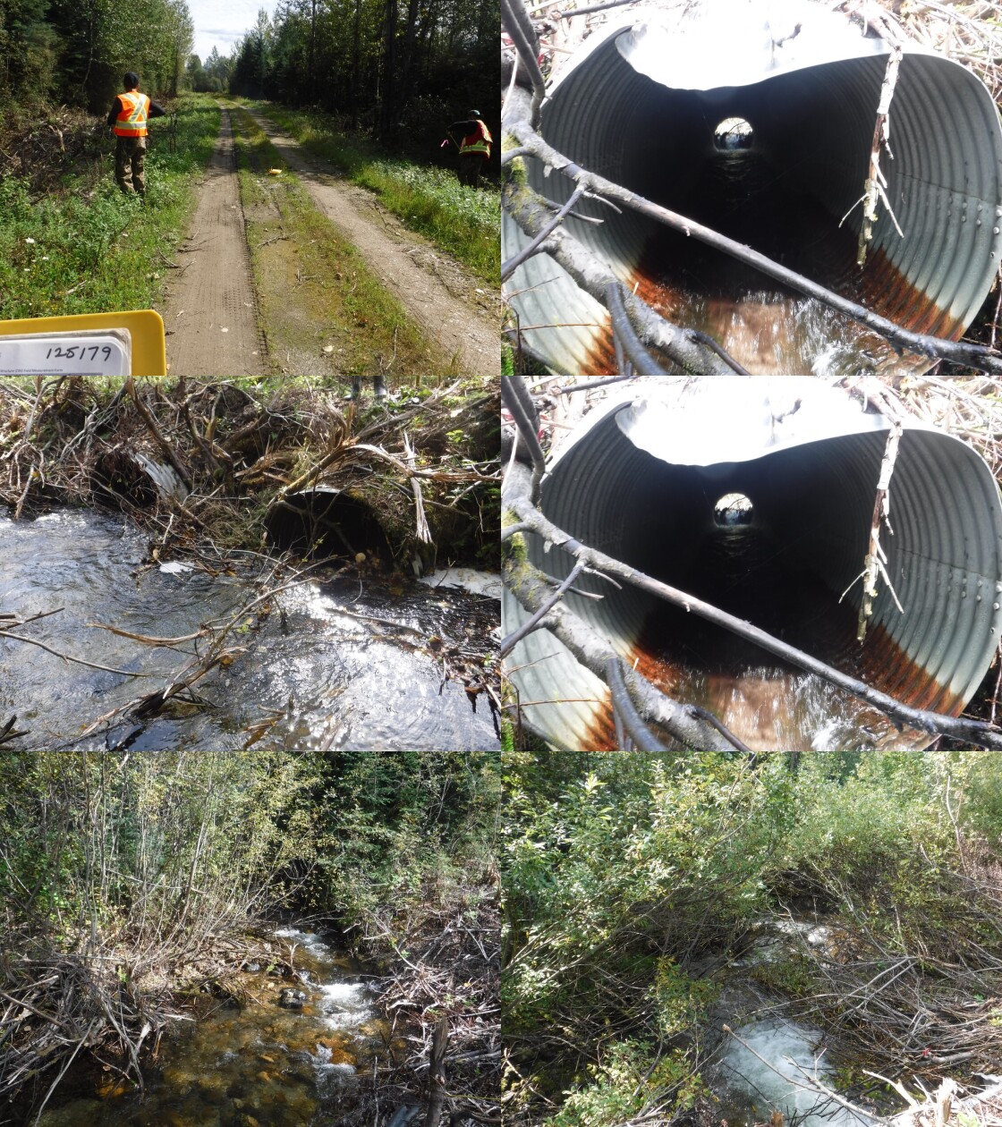
Figure 3.3: Photos of crossing 125179 in 2019.
my_photo2 = fpr::fpr_photo_pull_by_str(str_to_pull = 'crossing_all', site = 125179)

my_caption2 = paste0('Photos of crossing ', my_site, ' in 2022.')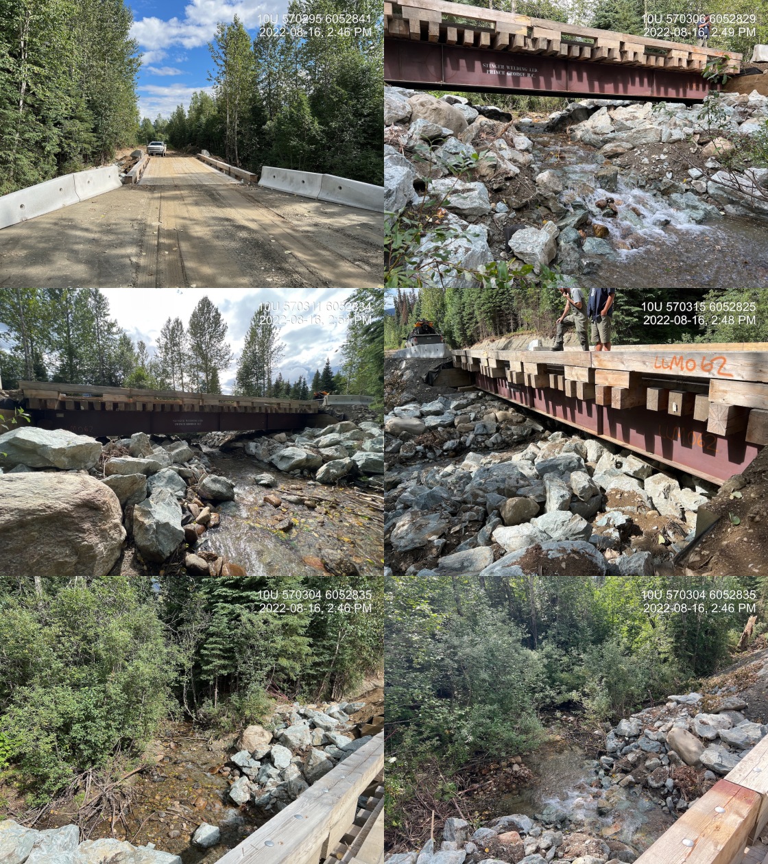
Figure 3.4: Photos of crossing 125179 in 2022.
my_caption <- paste0('Left: ', my_caption1, ' Right: ', my_caption2)

knitr::include_graphics(my_photo1)
knitr::include_graphics("fig/pixel.png")
knitr::include_graphics(my_photo2)
model_url <- '<iframe src="https://www.mapsmadeeasy.com/maps/public/8e3a0c68656c4480a66e067a6e14c0d3" scrolling="no" title="Maps Made Easy" width="100%" height="500" frameBorder ="0"></iframe>'
knitr::asis_output(model_url)my_photo = 'fig/pixel.png'
my_caption = paste0('Orthomosaic of bridge on Tributary to Missinka River. To zoom press "shift" and scroll.')
knitr::include_graphics(my_photo, dpi = NA)Figure 3.5: Orthomosaic of bridge on Tributary to Missinka River. To zoom press “shift” and scroll.
model_url <- '<iframe src="https://www.mapsmadeeasy.com/maps/public_3D/8e3a0c68656c4480a66e067a6e14c0d3" scrolling="no" title="Maps Made Easy" width="100%" height="500" frameBorder ="0"></iframe>'

knitr::asis_output(model_url)
my_photo = 'fig/pixel.png'
my_caption = paste0('3D model of newly installed bridge on a tributary to Missinka Creek. ')
knitr::include_graphics(my_photo, dpi = NA)Figure 3.6: 3D model of newly installed bridge on a tributary to Missinka Creek.
Recommendations
It is recommended that future monitoring be conducted at this location to track the stream morphological changes and provide insight into fish migration within the system. Electrofishing with tagging of target species is recommended along with photo documentation of stream morphology near the bridge. Fish sampling in the adjacent similar sized stream (PSCIS crossing 125180) containing culverts ranked as barriers would provide reference site data for comparison.
Designs
Three engineering designs for structure replacements with bridges were commissioned in 2022/23. Additionally, British Columbia Timber Sales is planning to deactivate the Chuchinka-Colbourne FSR between the location of 125345 (Tributary to Parsnip River) and the Chuckhinka-Anzac FSR (pers comm. Stephanie Sundquist, BCTS Planning Forester). The work was scheduled for July and August of 2022 but was delayed until 2023 due to a road washout in 2022. BCTS was able to obtain funding for the work through the Forest Carbon Initiative and the work will include a full road rehabilitation as well as decompaction and replanting.
Sinclar Forest Group commissioned a design for PSCIS crossing 125000 on a tributary to the Parsnip River 2km upstream of the confluence with the Parsnip River, on the Chuchinka-Arctic FSR approximately 9km north-west of the outlet of Arctic Lake. Plans were in place for remediation of the site in 2023/24 with funding support from FWCP however in the spring of 2023 Sinclar indicated that updates to that road no longer made sense as most plans for logging beyond the stream were on hold due to old growth referrals. The British Columbia government has asked licensees to defer harvest of these areas until “partners develop a new approach for old growth forest management”. The design was paid for by Sinclar and was not reimbursed through FWCP. The site was assessed in the summer of 2022 with aerial imagery acquired by drone and fish sampling conducted. Results from those assessments are presented below in the section title Tributary to Parsnip River - PSCIS crossing 125000.
Canfor Forest Products Ltd. (Canfor) has commissioned designs for two sites on the Chuchinka-Table FSR that are planned for remediation:
- PSCIS crossing 125231 is located on a tributary to the Table River near the 21km mark of the Chuchinka-Table FSR. The culvert is located 0.7km from the confluence of the Table River on the upstream side of the CN Railway where a crossing considered passable is located. The subject stream flows into the Table River at a point 7.9 km upstream from the confluence with the Parsnip River. Detailed information regarding the site is located in the report by A. Irvine (2020) which can be found here.
- The second site is Fern Creek (PSCIS 125261) located at km 2.1 of the Chuchinka-Table FSR. This site was prioritized through the interactive dashboard included in the 2021 reporting from this project (A. Irvine 2022) and 2022 field surveys. Details are presented in Fern Creek - PSCIS crossing 125261. FWCP funds from 2022/2023 ficsal were used by Canfor to purchase materials for future construction at both sites. In addition to designs, Canfor has contracted DWB Engineering to complete environmental management plans and permit the projects.
Habitat Confirmation Assessments
Tributary to Anzac River - PSCIS crossing 6745
PSCIS crossing 6745 is located on a tributary to Anzac River, on Chuchinka-Crocker FSR. This site is located approximately 0.9km upstream from the confluence with the Anzac River. The confluence is located at km 10.7 of the Anzac River. At crossing 6745, tributary to Anzac River is a third order stream with a watershed area upstream of the crossing of approximately 2.1km2. The elevation of the watershed ranges from a maximum of 869m to 745m near the crossing (Table 3.1). At the time of reporting, there was no fisheries information available within provincial databases for the area upstream of crossing 6745.
The Anzac River is one of the main tributaries to the Parsnip River. It is a 78km long tributary and drains a 939km2 watershed. The average gradient ranges from 1-2% in the upper reaches to a gradient less than 0.5% in the unconfined areas in the valley flats. In the Anzac River, a 30-km stretch from a chute obstruction at 47 km to 16 km is assumed to provide productive summer rearing habitats for adult as it is characterized by a high abundance of Arctic Grayling (Hagen and Stamford 2021; Hagen, Pillipow, and Gantner 2019).
fpr::fpr_table_wshd_sum(site_id = my_site) %>%
  fpr::fpr_kable(caption_text = paste0('Summary of derived upstream watershed statistics for PSCIS crossing ', my_site, '.'),
           footnote_text = 'Elev P60 = Elevation at which 60% of the watershed area is above',
scroll = F)| Site | Area Km | Elev Site | Elev Min | Elev Max | Elev Median | Elev P60 | Aspect |
|---|---|---|---|---|---|---|---|
| 6745 | 2.1 | 764 | 745 | 869 | 835 | 831 | WSW |
| * Elev P60 = Elevation at which 60% of the watershed area is above |
A summary of habitat modelling outputs is presented in Table 3.2 and a map of the watershed is provided in map attachment 093J.124.
| Habitat | Potential | Remediation Gain | Remediation Gain (%) |
|---|---|---|---|
| BT Rearing (km) | 1.2 | 0.6 | 50 |
| BT Spawning (km) | 0.0 | 0.0 | – |
| BT Network (km) | 6.1 | 6.1 | 100 |
| BT Stream (km) | 3.7 | 3.7 | 100 |
| BT Lake Reservoir (ha) | 0.0 | 0.0 | – |
| BT Wetland (ha) | 0.0 | 0.0 | – |
| BT Slopeclass03 (km) | 2.7 | 2.7 | 100 |
| BT Slopeclass05 (km) | 1.0 | 1.0 | 100 |
| BT Slopeclass08 (km) | 0.0 | 0.0 | – |
| BT Slopeclass15 (km) | 0.1 | 0.1 | 100 |
| * Model data is preliminary and subject to adjustments. |
Stream Characteristics at Crossing
At the time of the survey, PSCIS crossing 6745 was un-embedded, non-backwatered and ranked as a potential barrier to upstream fish passage according to the provincial protocol (MoE 2011) (Table 3.3). Water temperature was 11\(^\circ\)C, pH was 7.9 and conductivity was 102uS/cm.
| Location and Stream Data |
|
Crossing Characteristics | – |
|---|---|---|---|
| Date | 2022-08-14 | Crossing Sub Type | Round Culvert |
| PSCIS ID | 6745 | Diameter (m) | 1.6 |
| External ID | – | Length (m) | 14 |
| Crew | MW AI | Embedded | No |
| UTM Zone | 10 | Depth Embedded (m) | – |
| Easting | 533992 | Resemble Channel | No |
| Northing | 6076165 | Backwatered | No |
| Stream | tributary to Anzac River | Percent Backwatered | – |
| Road | Chuchinka-Crocker FSR | Fill Depth (m) | 0.6 |
| Road Tenure | Resource Demographic | Outlet Drop (m) | 0 |
| Channel Width (m) | 1.5 | Outlet Pool Depth (m) | 0 |
| Stream Slope (%) | 2 | Inlet Drop | No |
| Beaver Activity | No | Slope (%) | 1 |
| Habitat Value | Medium | Valley Fill | Deep Fill |
| Final score | 15 | Barrier Result | Potential |
| Fix type | Replace Structure with Streambed Simulation CBS | Fix Span / Diameter | 3 |
Photos: From top left clockwise: Road/Site Card, Barrel, Outlet, Downstream, Upstream, Inlet.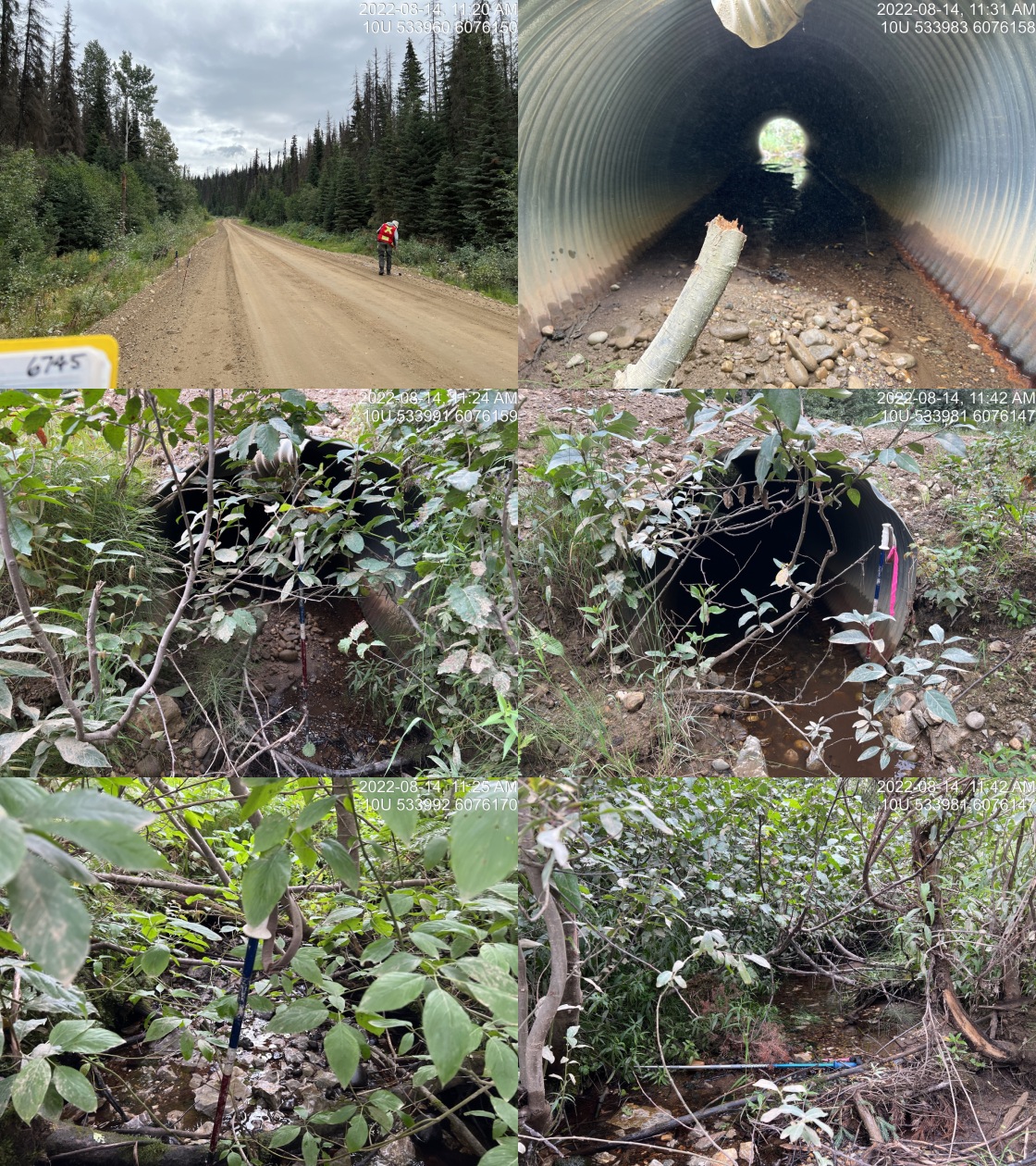
|
|||
| Comments: Damaged near outlet. Small stream but flowing. Middle of pipe filled with fines. 11:18 |
Stream Characteristics Downstream
The stream was surveyed downstream from crossing 6745 for 200m (Figures 3.7 - 3.8). The average channel width was 1.2m, the average wetted width was 1m, and the average gradient was 0.5%.The dominant substrate was gravels with fines sub-dominant.Total cover amount was rated as abundant with undercut banks dominant. Cover was also present as small woody debris, large woody debris, and overhanging vegetation. There were pockets of gravels suitable for resident salmonid spawning. Habitat was rated as medium value for salmonid rearing and spawning with relatively low flow volumes and no deep pools.
Stream Characteristics Upstream
The stream was surveyed upstream from crossing 6745 for 550m (Figures 3.9 - 3.10). The average channel width was 1.5m, the average wetted width was 1m, and the average gradient was 1.7%.The dominant substrate was gravels with fines sub-dominant.Total cover amount was rated as moderate with undercut banks dominant. Cover was also present as small woody debris, large woody debris, deep pools, and overhanging vegetation. There were abundant gravels present, suitable for resident rainbow spawning. Some deep pools up to 45cm in depth were present that would be suitable for rearing and potentially overwintering. Overall, the habitat surveyed upstream of the crossing was rated as medium value containing habitat suitable for spawning and rearing salmonids.
Conclusion
Modelling indicates there is 1.2km of habitat upstream of crossing 6745 suitable for bull trout rearing with areas surveyed rated as medium value for rearing and spawning. Crossing 6745 was ranked as a low priority for proceeding to design for replacement. The culvert is considered a potential barrier but may not be a fish passage issue during all but highest flow levels. Fish sampling could be conducted to to determine fish presence upstream and downstream of the crossing.
tab_hab_summary %>%
  filter(Site  == my_site) %>%
  # select(-Site) %>%
  fpr::fpr_kable(caption_text = paste0('Summary of habitat details for PSCIS crossing ', my_site, '.'),
scroll = F) | Site | Location | Length Surveyed (m) | Channel Width (m) | Wetted Width (m) | Pool Depth (m) | Gradient (%) | Total Cover | Habitat Value |
|---|---|---|---|---|---|---|---|---|
| 6745 | Downstream | 200 | 1.2 | 1 | – | 0.5 | abundant | medium |
| 6745 | Upstream | 550 | 1.5 | 1 | 0.3 | 1.7 | moderate | medium |
my_photo1 = fpr::fpr_photo_pull_by_str(str_to_pull = '_d1_')

my_caption1 = paste0('Typical habitat downstream of PSCIS crossing ', my_site, '.')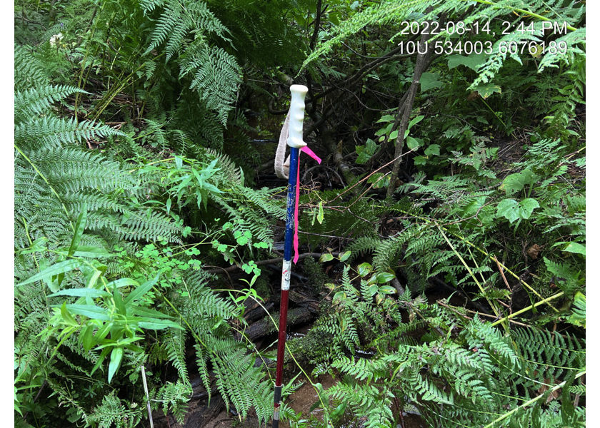
Figure 3.7: Typical habitat downstream of PSCIS crossing 6745.
my_photo2 = fpr::fpr_photo_pull_by_str(str_to_pull = '_d2_')

my_caption2 = paste0('Typical habitat downstream of PSCIS crossing ', my_site, '.')
Figure 3.8: Typical habitat downstream of PSCIS crossing 6745.
my_caption <- paste0('Left: ', my_caption1, ' Right: ', my_caption2)

knitr::include_graphics(my_photo1)
knitr::include_graphics("fig/pixel.png")
knitr::include_graphics(my_photo2)
my_photo1 = fpr::fpr_photo_pull_by_str(str_to_pull = '_u1_')
my_caption1 = paste0('Typical habitat upstream of PSCIS crossing ', my_site, '.')
Figure 3.9: Typical habitat upstream of PSCIS crossing 6745.
my_photo2 = fpr::fpr_photo_pull_by_str(str_to_pull = '_u2_')

my_caption2 = paste0('Typical habitat upstream of PSCIS crossing ', my_site, '.')
Figure 3.10: Typical habitat upstream of PSCIS crossing 6745.
my_caption <- paste0('Left: ', my_caption1, ' Right: ', my_caption2)

knitr::include_graphics(my_photo1)
knitr::include_graphics("fig/pixel.png")
knitr::include_graphics(my_photo2)
Tributary to Parsnip River - PSCIS crossing 125000
PSCIS crossing 125000 is located on a tributary to Parsnip River, approximately 2km upstream of the confluence with the Parsnip River, on the Chuchinka-Arctic FSR approximately 9km north-west of the outlet of Arctic Lake. Arctic Lake is located within Arctic Pacific Lakes Provincial Park and has an area of 112ha. The park has significant historical and recreational values and contains Mcleod Lake Indian Band reservation lands (Arctic Lake 10). The lake supports a diverse population of fish, including lake trout, bull trout, rainbow trout, kokanee, dolly varden, mountain whitefish, redside shiner, lake char, and chinook salmon, and arctic grayling (BC Parks 2020). There are no other stream crossings on the mainstem of this stream that block fish passage. Rainbow trout and sculpin have been captured in the past both upstream and downstream of the crossing. A map of the watershed is provided in map attachment 93I.111.
PSCIS crossing 125000 was ranked as a high priority for remediation following habitat confirmations done by A. Irvine (2020) in 2019. At that time, it was estimated that there was 3.5km of habitat with a gradient less than 5% available upstream of the crossing. Habitat was rated as high value for salmonid rearing and spawning. Fish sampling (minnowtrapping) in 2019 confirmed that rainbow trout and sculpin were present downstream of the crossing however no fish were captured upstream. At the time of survey in 2019, the culvert was a complete barrier to upstream fish passage, having an outlet drop of 0.4m and a outlet pool depth of 1.5m. A detailed overview of stream characteristics and habitat details can be found in the 2019 report.
Plans were in place for remediation of the site in 2022/2023 and 2023/24 with funding support from FWCP however in the spring of 2023 Sinclar indicated that updates to the road no longer made sense as most plans for logging beyond the stream were on hold due to old growth referrals (Figure 3.11). The British Columbia government has asked licensees to defer harvest of these areas until “partners develop a new approach for old growth forest management” (Ministry of Forests n.d.).
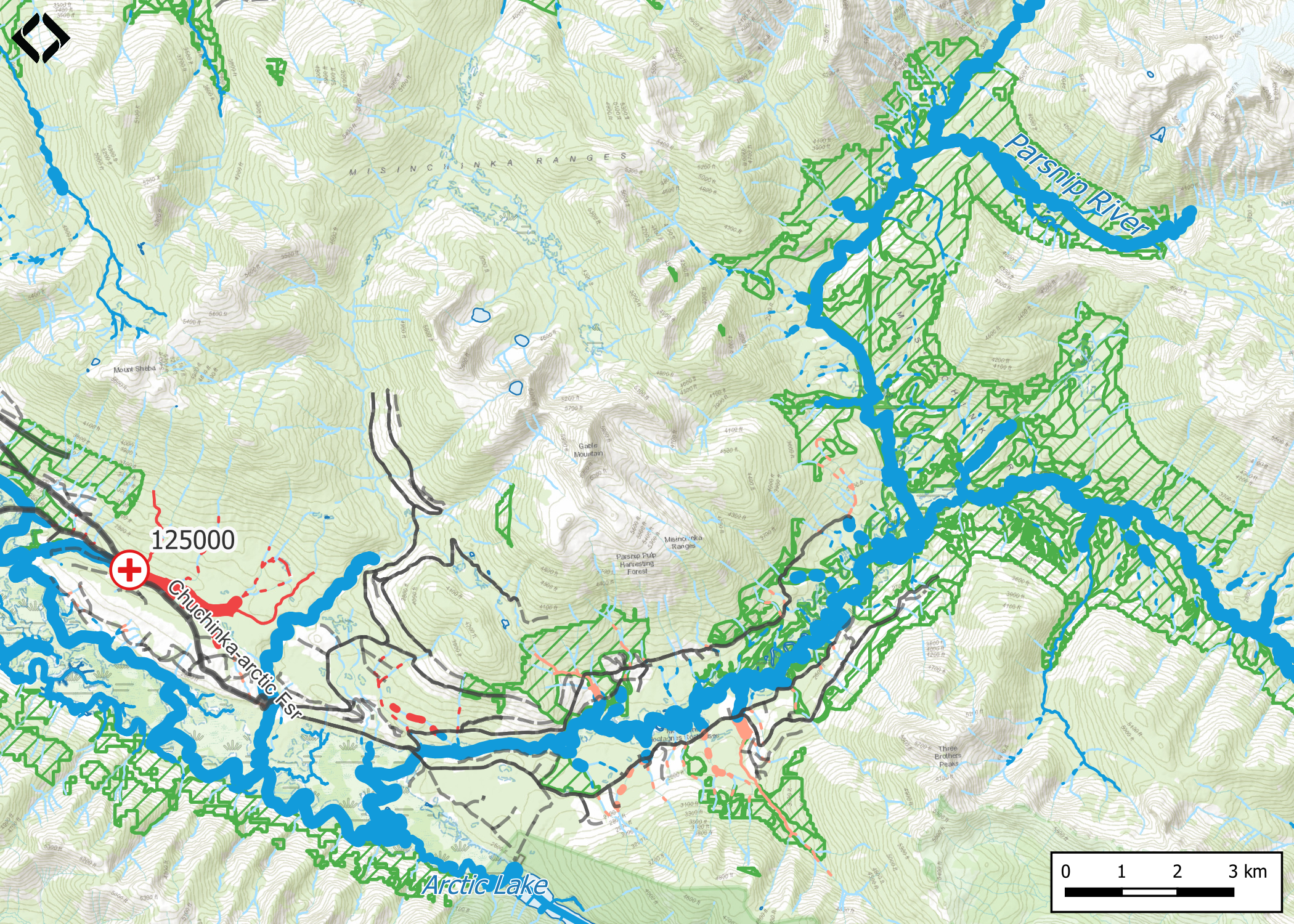
Figure 3.11: Map showing old growth management areas (green hashed polygons) beyond crossing 125000 accessed by the Chuckinka-Arctic FSR
This site was reassessed in 2022, with drone survey and fish sampling conducted. At the time of survey the crossing was un-embedded, non-backwatered and ranked as a barrier to upstream fish passage. The culvert was undersized - evidenced by the large outlet drop of 0.6m and outlet pool depth of 2m (MoE 2011) (Table 3.5).
| Location and Stream Data |
|
Crossing Characteristics | – |
|---|---|---|---|
| Date | 2022-08-15 | Crossing Sub Type | Round Culvert |
| PSCIS ID | 125000 | Diameter (m) | 1.5 |
| External ID | – | Length (m) | 18 |
| Crew | MW AI | Embedded | No |
| UTM Zone | 10 | Depth Embedded (m) | – |
| Easting | 577540 | Resemble Channel | No |
| Northing | 6038199 | Backwatered | No |
| Stream | Tributary to Parsnip River | Percent Backwatered | – |
| Road | Chuchinka-Arctic FSR | Fill Depth (m) | 2.5 |
| Road Tenure | Resource Demographic | Outlet Drop (m) | 0.6 |
| Channel Width (m) | 4.52 | Outlet Pool Depth (m) | 2 |
| Stream Slope (%) | 1.5 | Inlet Drop | No |
| Beaver Activity | No | Slope (%) | 2 |
| Habitat Value | Medium | Valley Fill | Deep Fill |
| Final score | 34 | Barrier Result | Barrier |
| Fix type | Replace with New Open Bottom Structure | Fix Span / Diameter | 15 |
Photos: From top left clockwise: Road/Site Card, Barrel, Outlet, Downstream, Upstream, Inlet.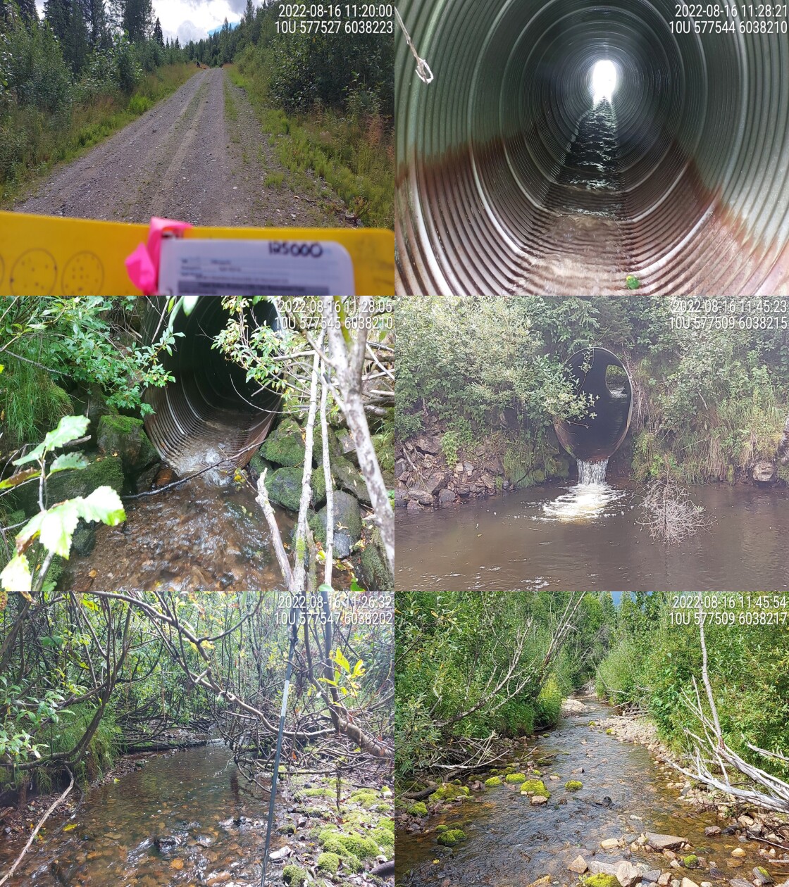
|
|||
| Comments: Habitat survey done with drone. 11:15:00 AM |
# this data is not correct so turned chunk off
# At crossing `r as.character(my_site)`, this tributary to Parsnip River is a `r fpr::fpr_my_bcfishpass() %>% english::ordinal()` order stream with a watershed area upstream of the crossing of approximately `r fpr::fpr_my_wshd()`km^2^. The elevation of the watershed ranges from a maximum of `r fpr::fpr_my_wshd(col = 'elev_max')`m to `r fpr::fpr_my_wshd(col = 'elev_min')`m near the crossing (Table
\@ref(tab:tab-wshd-125000)).
fpr::fpr_table_wshd_sum(site_id = my_site) %>%
  fpr::fpr_kable(caption_text = paste0('Summary of derived upstream watershed statistics for PSCIS crossing ', my_site, '.'),
           footnote_text = 'Elev P60 = Elevation at which 60% of the watershed area is above',
           scroll = F)
# this data is incorrect becasue needed to go to old db so turned off
fpr::fpr_table_bcfp(scroll = F) Aerial Imagery
In 2019 a video survey was conducted by drone and can be viewed here. In the summer of 2022, additional surveys were conducted with a remotely piloted aircraft at the crossing with resulting images stitched into an orthomosaic and 3-dimensional model presented in Figures 3.12 - 3.13.
model_url <- '<iframe src="https://www.mapsmadeeasy.com/maps/public/0b96f06f52be467db7250b3caeeecee3" scrolling="no" title="Maps Made Easy" width="100%" height="500" frameBorder ="0"></iframe>'

knitr::asis_output(model_url)
my_photo = 'fig/pixel.png'
my_caption = paste0('Orthomosaic of site of planned bridge on tributary to Parsnip River. To zoom press "shift" and scroll.')
knitr::include_graphics(my_photo, dpi = NA)Figure 3.12: Orthomosaic of site of planned bridge on tributary to Parsnip River. To zoom press “shift” and scroll.
model_url <- '<iframe src="https://www.mapsmadeeasy.com/maps/public_3D/0b96f06f52be467db7250b3caeeecee3" scrolling="no" title="Maps Made Easy" width="100%" height="500" frameBorder ="0"></iframe>'

knitr::asis_output(model_url)
my_photo = 'fig/pixel.png'
my_caption = paste0('3D model of crossing 125000 where newly installed bridge is planned on a tributary to Parsnip River. To zoom press "shift" and scroll.')
knitr::include_graphics(my_photo, dpi = NA)Figure 3.13: 3D model of crossing 125000 where newly installed bridge is planned on a tributary to Parsnip River. To zoom press “shift” and scroll.
Fish Sampling
Electrofishing was conducted at the site with results summarised in Tables 3.6 - 3.7 and Figure 3.14. Rainbow trout and sculpin were captured both upstream and downstream of the crossing. Rainbow trout over 60mm in length were tagged using Passive Integrated Transponders (PIT) so health and movement can be tracked over time. Fish sampling data and tag information can be referenced here.
| site | passes | ef_length_m | ef_width_m | area_m2 | enclosure |
|---|---|---|---|---|---|
| 125000_ds_ef1 | 1 | 28 | 3.2 | 89.6 | Open |
| 125000_ds_ef2 | 1 | 7 | 3.0 | 21.0 | Open |
| 125000_ds_ef3 | 1 | 5 | 2.9 | 14.5 | Open |
| 125000_us_ef1 | 1 | 8 | 2.0 | 16.0 | Open |
| 125000_us_ef2 | 1 | 23 | 3.3 | 75.9 | Open |
| 125000_us_ef3 | 1 | 21 | 2.9 | 60.9 | Open |
| local_name | species_code | life_stage | catch | density_100m2 | nfc_pass |
|---|---|---|---|---|---|
| 125000_ds_ef1 | CC | fry | 3 | 3.3 | FALSE |
| 125000_ds_ef1 | CC | parr | 1 | 1.1 | FALSE |
| 125000_ds_ef1 | RB | fry | 20 | 22.3 | FALSE |
| 125000_ds_ef1 | RB | parr | 13 | 14.5 | FALSE |
| 125000_ds_ef1 | RB | juvenile | 3 | 3.3 | FALSE |
| 125000_ds_ef2 | CC | fry | 2 | 9.5 | FALSE |
| 125000_ds_ef2 | RB | fry | 3 | 14.3 | FALSE |
| 125000_ds_ef2 | RB | parr | 5 | 23.8 | FALSE |
| 125000_ds_ef3 | RB | fry | 1 | 6.9 | FALSE |
| 125000_ds_ef3 | RB | parr | 7 | 48.3 | FALSE |
| 125000_ds_ef3 | RB | juvenile | 1 | 6.9 | FALSE |
| 125000_us_ef1 | RB | fry | 2 | 12.5 | FALSE |
| 125000_us_ef1 | RB | parr | 1 | 6.2 | FALSE |
| 125000_us_ef1 | RB | adult | 1 | 6.2 | FALSE |
| 125000_us_ef2 | CC | parr | 1 | 1.3 | FALSE |
| 125000_us_ef2 | RB | fry | 2 | 2.6 | FALSE |
| 125000_us_ef2 | RB | parr | 1 | 1.3 | FALSE |
| 125000_us_ef2 | RB | juvenile | 5 | 6.6 | FALSE |
| 125000_us_ef3 | CC | fry | 1 | 1.6 | FALSE |
| 125000_us_ef3 | RB | fry | 1 | 1.6 | FALSE |
| 125000_us_ef3 | RB | parr | 4 | 6.6 | FALSE |
|
* nfc_pass FALSE means fish were captured in final pass indicating more fish of this species/lifestage may have remained in site. Mark-recaptured required to reduce uncertainties. |
my_caption <- paste0('Densites of fish (fish/100m2) captured upstream of PSCIS crossing ', my_site, '.')

fpr_plot_fish_box() 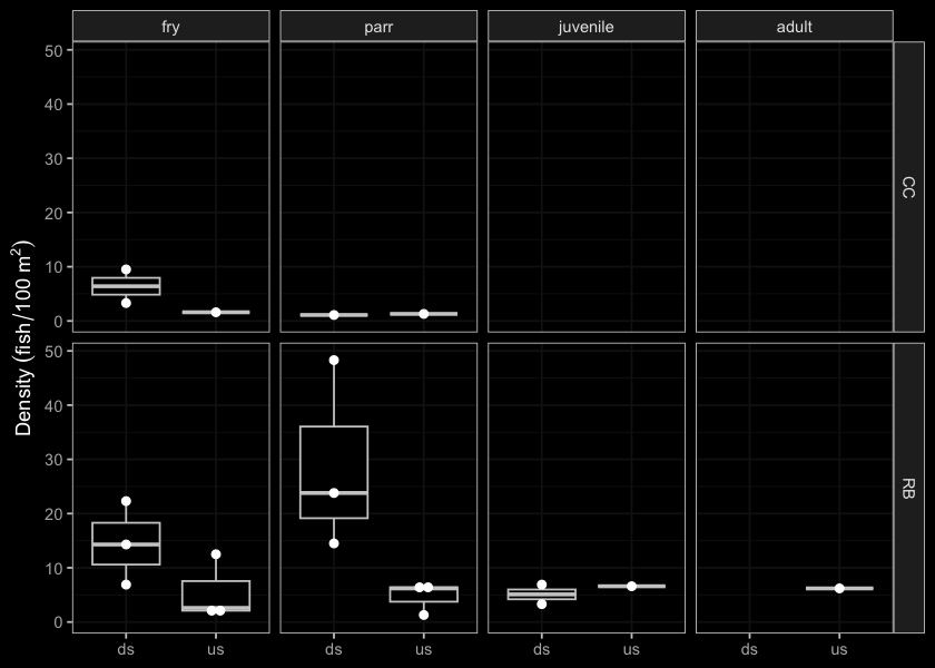
Figure 3.14: Densites of fish (fish/100m2) captured upstream of PSCIS crossing 125000.
Conclusion
Although at the time of reporting plans for replacement of this site had been delayed, future removal (or replacement) of the crossing is still recommended. Prelininary cost estimates for the work were estmitated at /$350,000 to /$400,000. Additionally, re-assessment of the site with electrofishing in the 2023 and/or 2024 will provide valuable information regarding fish health and migration at the site.
Tributary to Missinka River - PSCIS crossing 125194
PSCIS crossing 125194 is located on a tributary to Missinka River, on Chuchinka-Missinka FSR. The site is located approximately 0.6km upstream from the confluence with the Missinka River. At crossing 125194, tributary to Missinka River is a second order stream with a watershed area upstream of the crossing of approximately 2.7km2. The elevation of the watershed ranges from a maximum of 1432m to 740m near the crossing (Table 3.8). Although there are numerous modelled crossings upstream of the subject culvert on the mainstem of the streawm, review of aerial imagery indicates that none of them are present. At the time of reporting, there was no fisheries information available for the area upstream of the crossing.
fpr::fpr_table_wshd_sum(site_id = my_site) %>%
  fpr::fpr_kable(caption_text = paste0('Summary of derived upstream watershed statistics for PSCIS crossing ', my_site, '.'),
           footnote_text = 'Elev P60 = Elevation at which 60% of the watershed area is above',
scroll = F)| Site | Area Km | Elev Site | Elev Min | Elev Max | Elev Median | Elev P60 | Aspect |
|---|---|---|---|---|---|---|---|
| 125194 | 2.7 | 828 | 740 | 1432 | 936 | 914 | S |
| * Elev P60 = Elevation at which 60% of the watershed area is above |
A summary of habitat modelling outputs is presented in Table 3.9 and a map of the watershed is provided in map attachment 093J.115. Of note, the freshwater atlas erroneously indicates there are no wetland areas upstream of the crossing, however aerial imagery of the site shows that there are significant areas of wetland primarily caused by beaver activity.
| Habitat | Potential | Remediation Gain | Remediation Gain (%) |
|---|---|---|---|
| BT Rearing (km) | 2.0 | 0.8 | 40 |
| BT Spawning (km) | 1.4 | 0.8 | 57 |
| BT Network (km) | 4.5 | 4.5 | 100 |
| BT Stream (km) | 4.5 | 4.5 | 100 |
| BT Lake Reservoir (ha) | 0.0 | 0.0 | – |
| BT Wetland (ha) | 0.0 | 0.0 | – |
| BT Slopeclass03 (km) | 2.8 | 2.8 | 100 |
| BT Slopeclass05 (km) | 0.8 | 0.8 | 100 |
| BT Slopeclass08 (km) | 0.0 | 0.0 | – |
| BT Slopeclass15 (km) | 0.7 | 0.7 | 100 |
| * Model data is preliminary and subject to adjustments. |
Stream Characteristics at Crossing
At the time of survey, PSCIS crossing 125194 was un-embedded, non-backwatered and ranked as a barrier to upstream fish passage according to the provincial protocol (MoE 2011) (Table 3.10). Water temperature was 10\(^\circ\)C, pH was 8 and conductivity was 180uS/cm.
| Location and Stream Data |
|
Crossing Characteristics | – |
|---|---|---|---|
| Date | 2022-08-17 | Crossing Sub Type | Round Culvert |
| PSCIS ID | 125194 | Diameter (m) | 1.8 |
| External ID | – | Length (m) | 30 |
| Crew | MW AI | Embedded | No |
| UTM Zone | 10 | Depth Embedded (m) | – |
| Easting | 563293 | Resemble Channel | No |
| Northing | 6050578 | Backwatered | No |
| Stream | tributary to Missinka River | Percent Backwatered | – |
| Road | Chuchinka-Missinka FSR | Fill Depth (m) | 4 |
| Road Tenure | Resource Demographic | Outlet Drop (m) | 1.1 |
| Channel Width (m) | 2.4 | Outlet Pool Depth (m) | 0.3 |
| Stream Slope (%) | 2 | Inlet Drop | Yes |
| Beaver Activity | No | Slope (%) | 2 |
| Habitat Value | Medium | Valley Fill | Deep Fill |
| Final score | 37 | Barrier Result | Barrier |
| Fix type | Replace with New Open Bottom Structure | Fix Span / Diameter | 15 |
Photos: From top left clockwise: Road/Site Card, Barrel, Outlet, Downstream, Upstream, Inlet.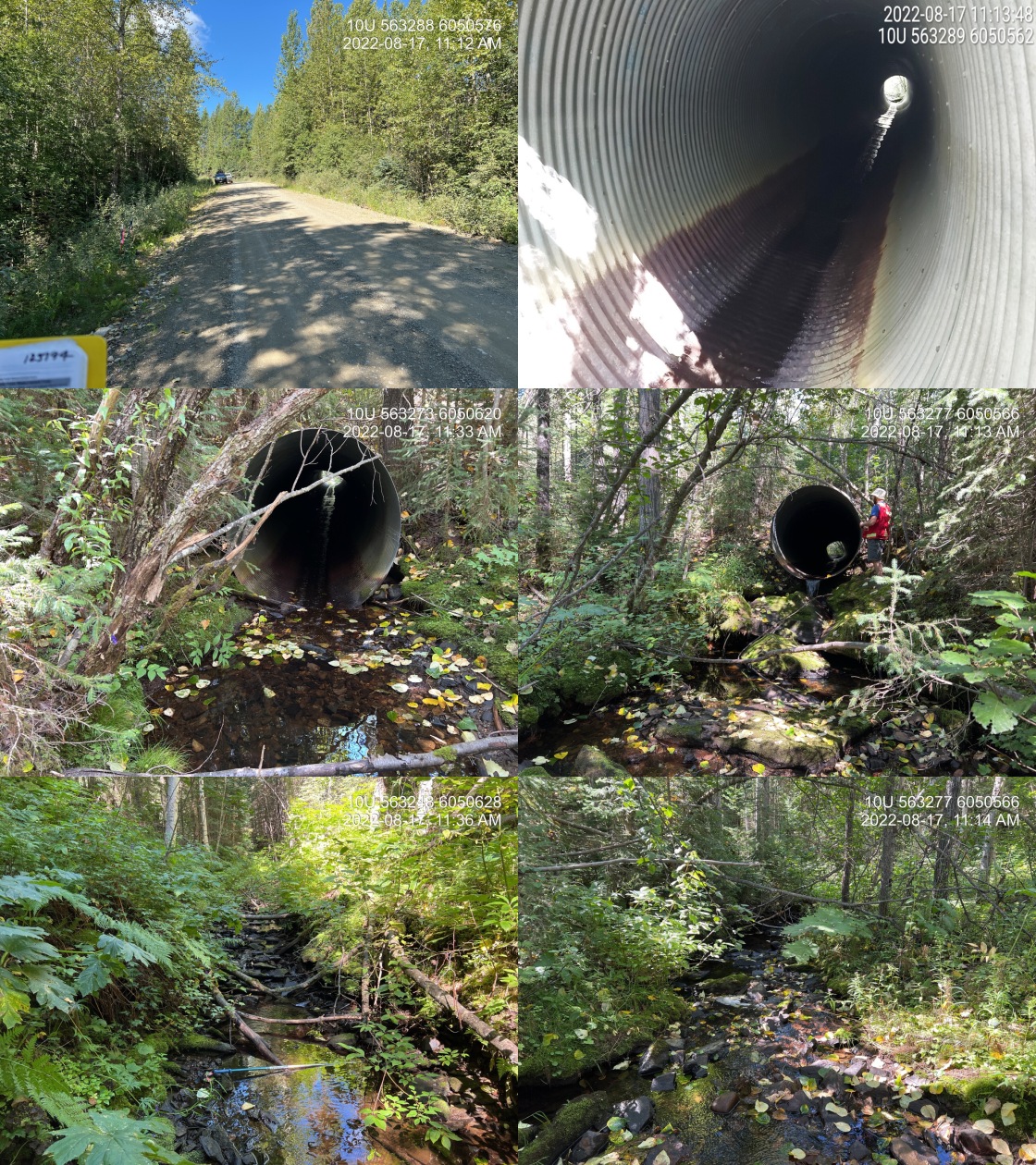
|
|||
| Comments: Very narrow cascade at outlet, big outlet drop. Good size pools downstream. Upstream has evenly distributed shale. Lots of functional woody debris. 11:09 |
Stream Characteristics Downstream
The stream was surveyed downstream from crossing 125194 for 250m (Figures 3.15 - 3.16). The dominant substrate was gravels with fines sub-dominant.Total cover amount was rated as moderate with small woody debris dominant. Cover was also present as large woody debris and overhanging vegetation.The average channel width was 2.8m, the average wetted width was 2.5m, and the average gradient was 2.8%. There were trace amounts of undercut banks and pools that were suitable for rearing. Abundant gravels were present that would be suitable for resident rainbow spawning. Habitat was reasonably complex due to abundant woody debris and rated as medium value for salmonid rearing and spawning.
Stream Characteristics Upstream
The stream was surveyed upstream from crossing 125194 for 500m (Figures 3.17 - 3.20). Total cover amount was rated as moderate with undercut banks dominant. Cover was also present as small woody debris, large woody debris, boulders, deep pools, and overhanging vegetation.The average channel width was 3.4m, the average wetted width was 2.5m, and the average gradient was 6.2%.The dominant substrate was cobbles with fines sub-dominant. The water was tinged brown at the time of survey; likely from beaver activity upstream. No gravels were present suitable for spawning in the area surveyed and the substrate was composed primarily of angular rock. Several rock steps 50-60cm high were present in the first 300m of survey that would prevent upstream juvenile salmonid migration. The location of modelled crossing 16601526 was accessed however no structure was present. There was however a large beaver dam approximately 1.6m in height at this location. Overall, the habitat surveyed upstream of the crossing was rated as medium value as a migration corridor containing suitable spawning habitat and having moderate rearing potential for rainbow trout.
Conclusion
Replacement of PSCIS crossing 125194 with a bridge (15m span) is recommended. The cost of the work was estimated at $375,000 for a cost benefit of 5333.3 linear m/$1000 and 6400 m2/$1000.
Crossing 125194 was ranked as a low priority for proceeding to design for replacement. Modelling indicates 2km of habitat upstream of crossing 125194 suitable for rainbow trout rearing with areas surveyed rated as medium value. Due to the beaver influenced wetland character upstream of the crossing the stream is not expected to provide habitat for bull trout. Remediation of the crossing would therefore likely benefit rainbow trout and sculpin species if they are present immediately downstream.
tab_hab_summary %>%
  filter(Site  == my_site) %>%
  # select(-Site) %>%
  fpr::fpr_kable(caption_text = paste0('Summary of habitat details for PSCIS crossing ', my_site, '.'),
scroll = F) | Site | Location | Length Surveyed (m) | Channel Width (m) | Wetted Width (m) | Pool Depth (m) | Gradient (%) | Total Cover | Habitat Value |
|---|---|---|---|---|---|---|---|---|
| 125194 | Downstream | 250 | 2.8 | 2.5 | 0.3 | 2.8 | moderate | medium |
| 125194 | Upstream | 500 | 3.4 | 2.5 | 0.4 | 6.2 | moderate | medium |
my_photo1 = fpr::fpr_photo_pull_by_str(str_to_pull = '_d1_')

my_caption1 = paste0('Typical habitat downstream of PSCIS crossing ', my_site, '.')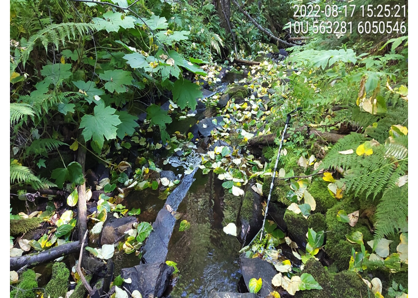
Figure 3.15: Typical habitat downstream of PSCIS crossing 125194.
my_photo2 = fpr::fpr_photo_pull_by_str(str_to_pull = '_d2_')

my_caption2 = paste0('Example of typical stream substrate downstream of PSCIS crossing ', my_site, '.')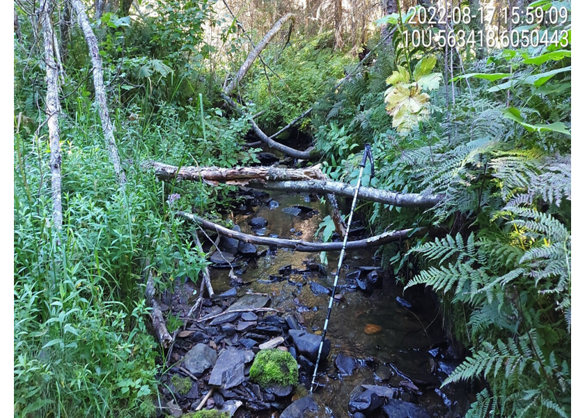
Figure 3.16: Example of typical stream substrate downstream of PSCIS crossing 125194.
my_caption <- paste0('Left: ', my_caption1, ' Right: ', my_caption2)

knitr::include_graphics(my_photo1)
knitr::include_graphics("fig/pixel.png")
knitr::include_graphics(my_photo2)
my_photo1 = fpr::fpr_photo_pull_by_str(str_to_pull = '_u1_')
my_caption1 = paste0('Typical habitat upstream of PSCIS crossing ', my_site, '.')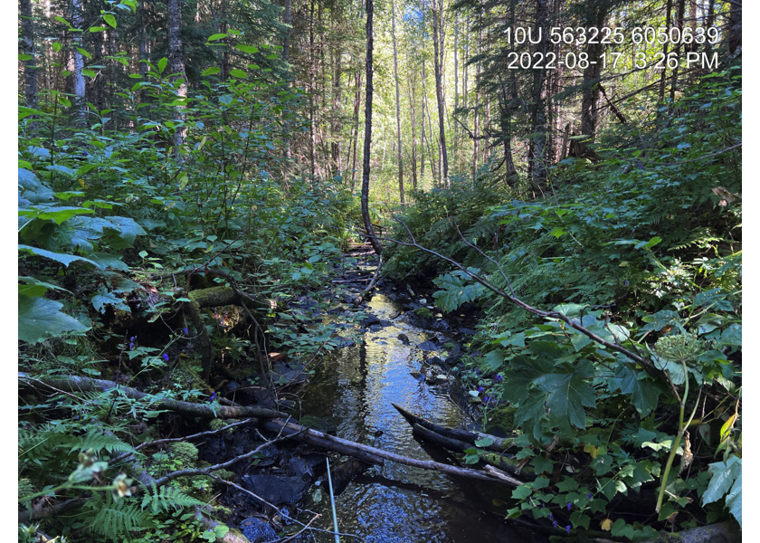
Figure 3.17: Typical habitat upstream of PSCIS crossing 125194.
my_photo2 = fpr::fpr_photo_pull_by_str(str_to_pull = '_u2_')

my_caption2 = paste0('Small rock step approximately 0.6m in height, upstream of PSCIS crossing ', my_site, '.')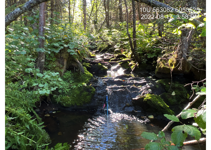
Figure 3.18: Small rock step approximately 0.6m in height, upstream of PSCIS crossing 125194.
my_caption <- paste0('Left: ', my_caption1, ' Right: ', my_caption2)

knitr::include_graphics(my_photo1)
knitr::include_graphics("fig/pixel.png")
knitr::include_graphics(my_photo2)
my_photo1 = fpr::fpr_photo_pull_by_str(str_to_pull = '_u3_')
my_caption1 = paste0('Typical habitat upstream of PSCIS crossing ', my_site, '.')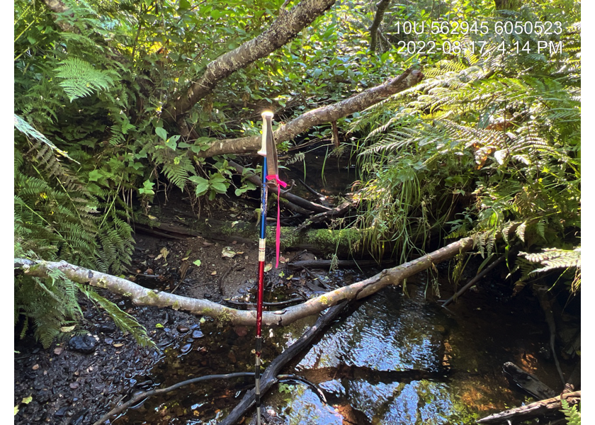
Figure 3.19: Typical habitat upstream of PSCIS crossing 125194.
my_photo2 = fpr::fpr_photo_pull_by_str(str_to_pull = '_u4_')

my_caption2 = paste0('Beaver dam 1.6m high at modelled crossing 16601526, upstream of PSCIS crossing ', my_site, '.')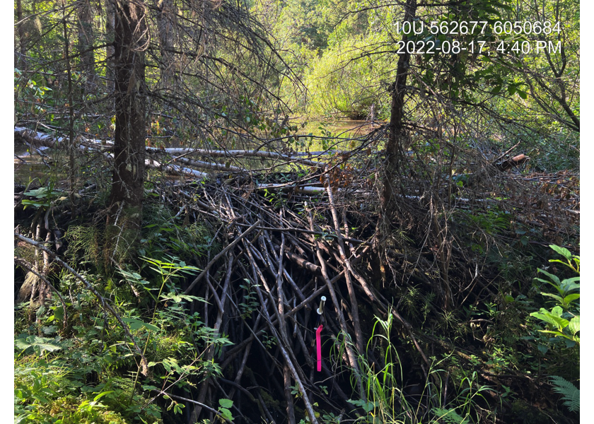
Figure 3.20: Beaver dam 1.6m high at modelled crossing 16601526, upstream of PSCIS crossing 125194.
my_caption <- paste0('Left: ', my_caption1, ' Right: ', my_caption2)

knitr::include_graphics(my_photo1)
knitr::include_graphics("fig/pixel.png")
knitr::include_graphics(my_photo2)
Fern Creek - PSCIS crossing 125261
PSCIS crossing 125261 is located on Fern Creek, approximately 0.3km upstream from the confluence with the Parsnip River, at km 2.1 on the Chuchinka-Table FSR. Canfor Corporation are the primary forest licensee at this location with the Ministry of Forests as the road tenure holders.
At crossing 125261, Fern Creek is a fourth order stream with a watershed area upstream of the crossing of approximately 23.5km2. The elevation of the watershed ranges from a maximum of 1137m to 730m near the crossing (Table 3.12). Fish species confirmed upstream of the FSR include burbot, rainbow trout, bull trout, sucker, reside shiner, dace and chub. A total of 148ha of lake and 37ha of wetland are modelled upstream. This includes Fern Lakes, a collection of three lakes that have a combined area of approximately 138ha. The outlet of the first lake in the chain is 3.3km upstream of the FSR.
PSCIS crossing 198321 was modelled as located on Fern Creek approximately 700m upstream of crossing 125261. However, upon visiting this location, this site was located at the end of an ATV trail and there was no structure or ford location. Additionally, the ATV trail did not continue beyond this point as the historic road was completely overgrown. There are several crossings modelled on the mainstem of Fern Creek upstream of the FSR however review of aerial imagery and deactivation of the road closer to that FSR provide significant weight of evidence that no crossing structures are present.
A summary of habitat modelling outputs is presented in Table 3.13 and a map of the watershed is provided in map attachment 093J.119.
# There are two other crossings (ID 16601842) modelled before the confluence with the lake closest to the FSR. One the mainstem of the stream and chain of lakes there are crossings modelled as between the first and second lakes (modelled_crossing_id 16600823) and between the second and third lakes (modelled_crossing_id 16600822). fpr::fpr_table_wshd_sum(site_id = my_site) %>%
fpr::fpr_kable(caption_text = paste0('Summary of derived upstream watershed statistics for PSCIS crossing ', my_site, '.'),
footnote_text = 'Elev P60 = Elevation at which 60% of the watershed area is above',
scroll = F)| Site | Area Km | Elev Site | Elev Min | Elev Max | Elev Median | Elev P60 | Aspect |
|---|---|---|---|---|---|---|---|
| 125261 | 23.5 | 730 | 723 | 1137 | 844 | 835 | SSW |
| * Elev P60 = Elevation at which 60% of the watershed area is above |
| Habitat | Potential | Remediation Gain | Remediation Gain (%) |
|---|---|---|---|
| BT Rearing (km) | 14.4 | 2.7 | 19 |
| BT Spawning (km) | 4.3 | 2.7 | 63 |
| BT Network (km) | 48.3 | 48.3 | 100 |
| BT Stream (km) | 38.4 | 38.4 | 100 |
| BT Lake Reservoir (ha) | 0.0 | 0.0 | – |
| BT Wetland (ha) | 0.0 | 0.0 | – |
| BT Slopeclass03 (km) | 7.2 | 7.2 | 100 |
| BT Slopeclass05 (km) | 14.9 | 14.9 | 100 |
| BT Slopeclass08 (km) | 3.9 | 3.9 | 100 |
| BT Slopeclass15 (km) | 11.5 | 11.5 | 100 |
| * Model data is preliminary and subject to adjustments. |
Stream Characteristics at Crossing
At the time of survey, PSCIS crossing 125261 was un-embedded, non-backwatered and ranked as a barrier to upstream fish passage according to the provincial protocol (MoE 2011) (Table 3.14). The culvert has baffles in it to assist upstream fish passage. However, at the time of survey, the baffles were not functioning properly as they were not effectively holding back substrate. Rip rap at the outlet was creating a cascade approximately 0.5m in height that could block the migration of younger resident fish, depending on flow velocities. Water temperature was 17\(^\circ\)C, pH was 8.4 and conductivity was 235uS/cm.
| Location and Stream Data |
|
Crossing Characteristics | – |
|---|---|---|---|
| Date | 2022-08-15 | Crossing Sub Type | Round Culvert |
| PSCIS ID | 125261 | Diameter (m) | 2.1 |
| External ID | – | Length (m) | 5 |
| Crew | MW AI | Embedded | No |
| UTM Zone | 10 | Depth Embedded (m) | – |
| Easting | 534600 | Resemble Channel | No |
| Northing | 6067770 | Backwatered | No |
| Stream | Fern Creek | Percent Backwatered | – |
| Road | Chuchinka-Table FSR | Fill Depth (m) | 0.8 |
| Road Tenure | Resource Demographic | Outlet Drop (m) | 0.4 |
| Channel Width (m) | 5.1 | Outlet Pool Depth (m) | 0.4 |
| Stream Slope (%) | 2 | Inlet Drop | No |
| Beaver Activity | No | Slope (%) | 1.5 |
| Habitat Value | High | Valley Fill | Deep Fill |
| Final score | 31 | Barrier Result | Barrier |
| Fix type | Replace with New Open Bottom Structure | Fix Span / Diameter | 15 |
Photos: From top left clockwise: Road/Site Card, Barrel, Outlet, Downstream, Upstream, Inlet.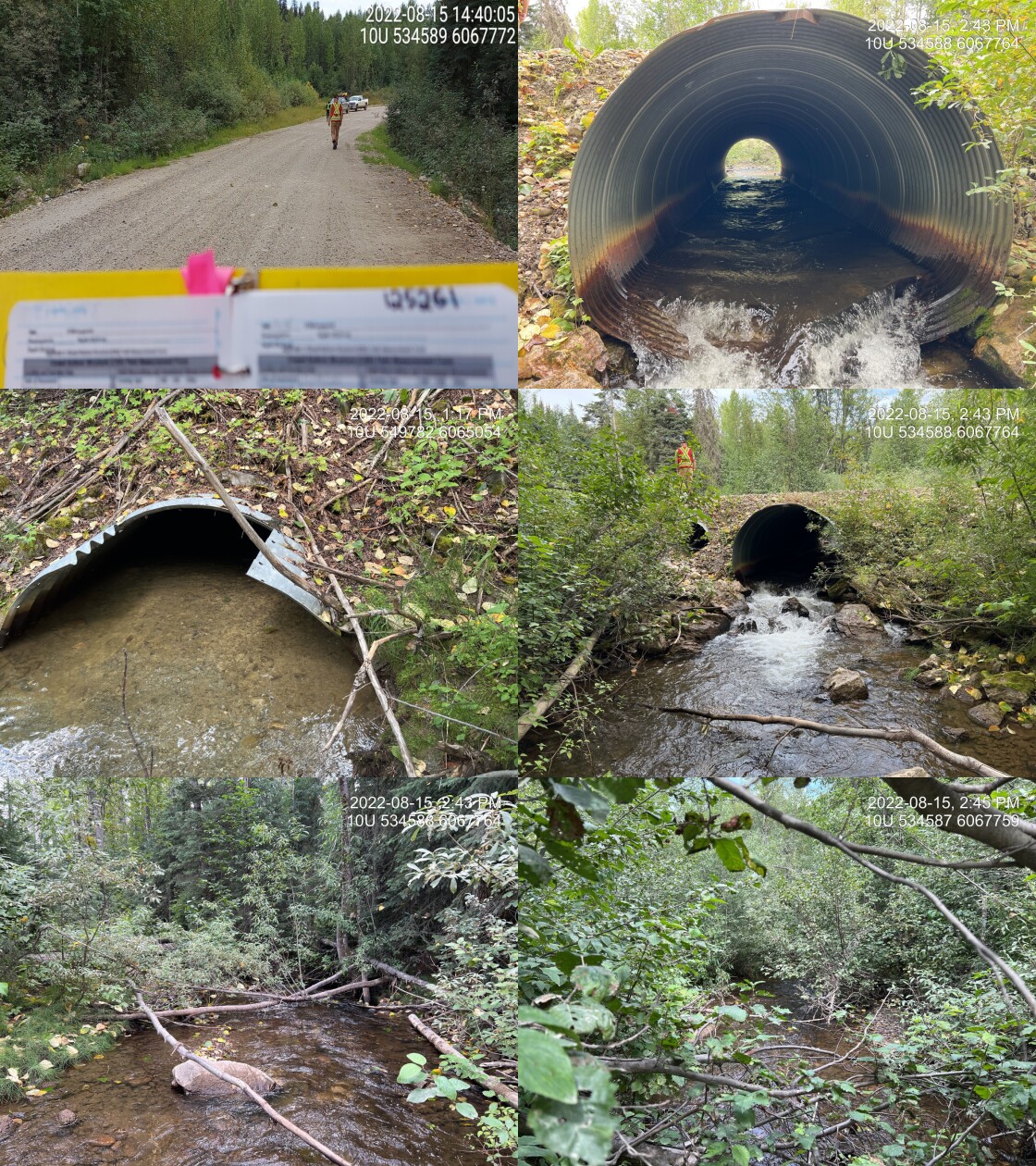
|
|||
| Comments: Culvert has baffles in it but has significant riprap at the outlet that creates cascade approximately 0.5 m high. 14:36 |
Stream Characteristics Downstream
The stream was surveyed downstream from crossing 125261 for 250m (Figures 3.21 - 3.22). The dominant substrate was gravels with fines sub-dominant.The average channel width was 5.6m, the average wetted width was 4.1m, and the average gradient was 1%.Total cover amount was rated as moderate with deep pools dominant. Cover was also present as small woody debris, overhanging vegetation, and instream vegetation. Extensive gravels were found in the first 150 m surveyed downstream. The habitat then transitioned to beaver influenced wetland, with depths of up to 1m and deep laminar flow. The habitat was rated as high value for salmonid rearing and spawning.
Stream Characteristics Upstream
The stream was surveyed upstream from crossing 125261 for 700m (Figures 3.23 - 3.26). Total cover amount was rated as moderate with deep pools dominant. Cover was also present as small woody debris, large woody debris, undercut banks, and overhanging vegetation.The dominant substrate was gravels with cobbles sub-dominant.The average channel width was 6.2m, the average wetted width was 2.4m, and the average gradient was 2.3%. This is a large stream with abundant gravel suitable for spawning and deep pools for overwintering. Numerous fish were observed, with complex habitat due to abundant large woody debris and deeply undercut banks. At the top end of the survey, the locaton of modelled crossing 16601271 was assessed. The crossing was not present as the road had been deactivated (Figures 3.27 - 3.28). Overall, the habitat surveyed upstream of crossing 125261 was rated as high value as an important migration corridor containing habitat suitable spawning habitat and high rearing potential.
Conclusion
Replacement of PSCIS crossing 125261 with a bridge (15m span) is recommended. The cost of the work was estimated at $375,000 for a cost benefit of 38373.3 linear m/$1000 and 97852 m2/$1000.
Modelling indicates that there is 14.4km of habitat upstream of crossing 125261 suitable for bull trout rearing with areas surveyed rated as high value for rearing and spawning. Crossing 125261 was ranked as a high priority for proceeding to design for replacement. Historic fisheries information upstream of the crossing indicate numerous species present including burbot and bull trout. As one of the larger tributaries in the area, this site is an excellent candidate for restoration. The presence of baffles within the pipe present at the time of assessment indicates that past efforts to facilitate connectivity have been pursued however the outlet drop and a lack of substrate in the pipe indicate those works are not functioning as intended. Although remediation of the site should be completed recommended regardless, it is recommended that if possible, Fern Creek be surveyed further upstream to confirm the presence (or absence) of road/stream crossing structures between crossing 125261 and Fern Lakes. Canfor has committed to replacement of the crossing in the coming years with an engineering design commissioned for the site in the spring of 2023. Additionally, materials for construction of the bridge (riprap) were purchased in the 2022/2023 fiscal to facilitate future works. It is recommended that electrofishing of the site be conducted prior to replacement of the site with PIT tagging of target species tagged (rainbow trout, bull trout and burbot). Additionally, baseline photo monitoring of stream morphology is recommended to track changes related to the works.
tab_hab_summary %>%
  filter(Site  == my_site) %>%
  # select(-Site) %>%
  fpr::fpr_kable(caption_text = paste0('Summary of habitat details for PSCIS crossing ', my_site, '.'),
scroll = F) | Site | Location | Length Surveyed (m) | Channel Width (m) | Wetted Width (m) | Pool Depth (m) | Gradient (%) | Total Cover | Habitat Value |
|---|---|---|---|---|---|---|---|---|
| 125261 | Downstream | 250 | 5.6 | 4.1 | 0.3 | 1.0 | moderate | high |
| 125261 | Upstream | 700 | 6.2 | 2.4 | 0.5 | 2.3 | moderate | high |
my_photo1 = fpr::fpr_photo_pull_by_str(str_to_pull = '_d1_')

my_caption1 = paste0('Habitat downstream of PSCIS crossing ', my_site, '.')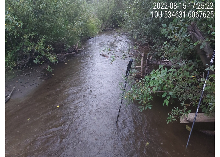
Figure 3.21: Habitat downstream of PSCIS crossing 125261.
my_photo2 = fpr::fpr_photo_pull_by_str(str_to_pull = '_d2_')

my_caption2 = paste0('Transition to wetland type habitat, downstream of PSCIS crossing ', my_site, '.')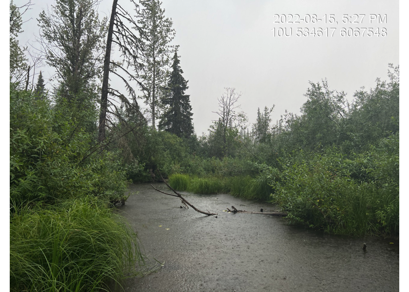
Figure 3.22: Transition to wetland type habitat, downstream of PSCIS crossing 125261.
my_caption <- paste0('Left: ', my_caption1, ' Right: ', my_caption2)

knitr::include_graphics(my_photo1)
knitr::include_graphics("fig/pixel.png")
knitr::include_graphics(my_photo2)
my_photo1 = fpr::fpr_photo_pull_by_str(str_to_pull = '_u1_')
my_caption1 = paste0('Habitat upstream of PSCIS crossing ', my_site, '.')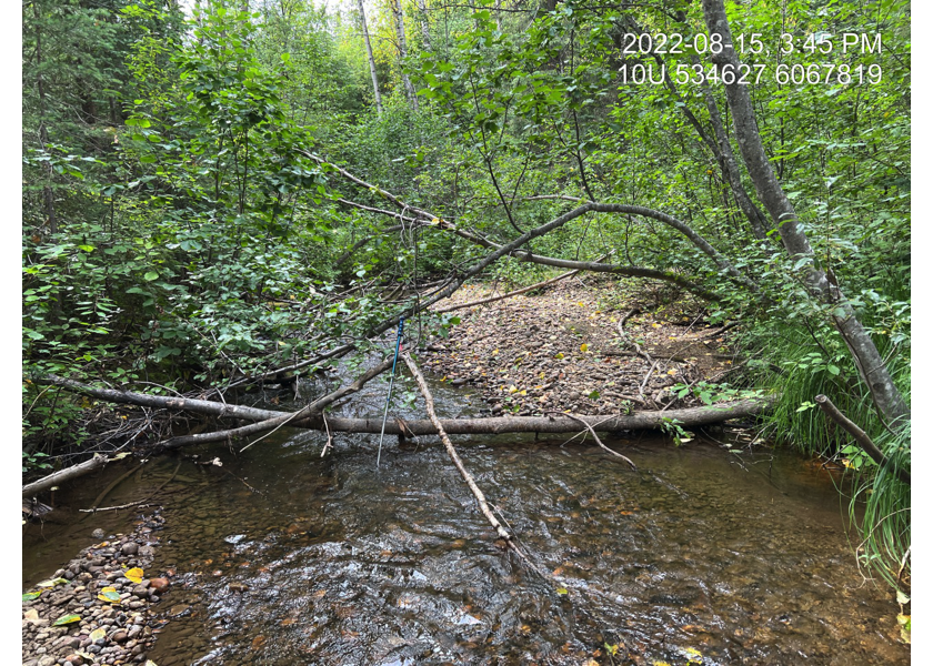
Figure 3.23: Habitat upstream of PSCIS crossing 125261.
my_photo2 = fpr::fpr_photo_pull_by_str(str_to_pull = '_u2_')

my_caption2 = paste0('Habitat upstream of PSCIS crossing ', my_site, '.')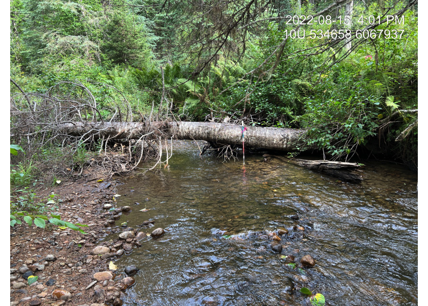
Figure 3.24: Habitat upstream of PSCIS crossing 125261.
my_caption <- paste0('Left: ', my_caption1, ' Right: ', my_caption2)

knitr::include_graphics(my_photo1)
knitr::include_graphics("fig/pixel.png")
knitr::include_graphics(my_photo2)
my_photo1 = fpr::fpr_photo_pull_by_str(str_to_pull = '_u3_')
my_caption1 = paste0('Deep pool and functional woody debris upstream of PSCIS crossing ', my_site, '.')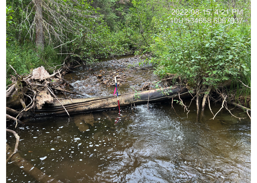
Figure 3.25: Deep pool and functional woody debris upstream of PSCIS crossing 125261.
my_photo2 = fpr::fpr_photo_pull_by_str(str_to_pull = '_u4_')

my_caption2 = paste0('Habitat upstream of PSCIS crossing ', my_site, '.')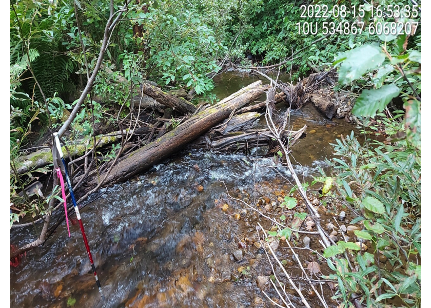
Figure 3.26: Habitat upstream of PSCIS crossing 125261.
my_caption <- paste0('Left: ', my_caption1, ' Right: ', my_caption2)

knitr::include_graphics(my_photo1)
knitr::include_graphics("fig/pixel.png")
knitr::include_graphics(my_photo2)
my_photo1 = fpr::fpr_photo_pull_by_str(site = my_site2, str_to_pull = '_downstream')
my_caption1 = paste0('Downstream view at end of survey, at location of PSCIC crossing 198321.')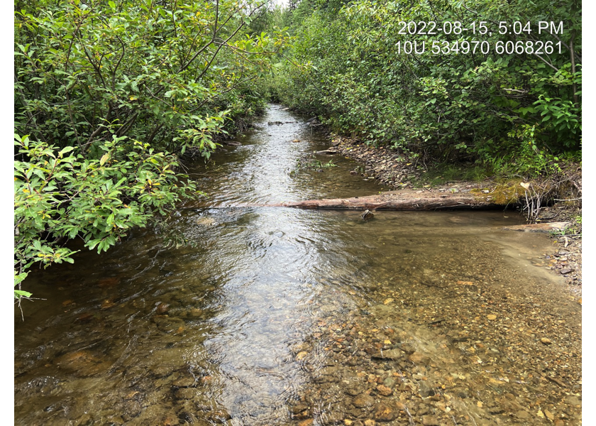
Figure 3.27: Downstream view at end of survey, at location of PSCIC crossing 198321.
my_photo2 = fpr::fpr_photo_pull_by_str(site = my_site2, str_to_pull = '_upstream')

my_caption2 = paste0('Upstream view at end of survey, at location of PSCIS crossing 198321.')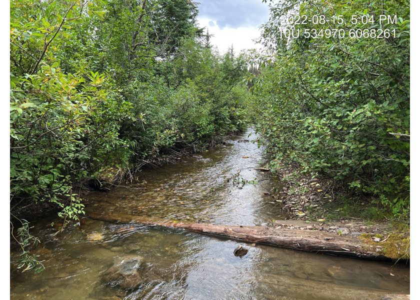
Figure 3.28: Upstream view at end of survey, at location of PSCIS crossing 198321.
my_caption <- paste0('Left: ', my_caption1, ' Right: ', my_caption2)

knitr::include_graphics(my_photo1)
knitr::include_graphics("fig/pixel.png")
knitr::include_graphics(my_photo2)
Fish Passage Assessments
Fish passage assessments were conducted at 12 sites in August 2022 by Allan Irvine, R.P.Bio., Mateo Winterscheidt, B.Sc., Nathan Prince, Traditional Land Use Coordinator - McLeod Lake and Eran Spence, Forestry Referrals Officer - McLeod Lake. Assessments were conducted at four previously unassessed sites, three assessments took place as part of habitat confirmation assessments and five sites were reassessed as they had either been replaced since the data in PSCIS was last updated or because they were being scoped for habitat values while serving as training case studies for collaborating technicians. All previously assessed crossings were either fords or bridges so presented no concerns for fish passage. Detailed data with photos are presented in Appendix - Phase 1 Fish Passage Assessment Data and Photos.