4 Results and Discussion
Results of Phase 1 and Phase 2 assessments are summarized in Figure 4.1 with additional details provided in sections below.
##make colors for the priorities
pal <-
   colorFactor(palette = c("red", "yellow", "grey", "black"),
               levels = c("high", "moderate", "low", "no fix"))

pal_phase1 <-
   colorFactor(palette = c("red", "yellow", "grey", "black"),
               levels = c("high", "moderate", "low", NA))

# tab_map_phase2 <- tab_map %>% filter(source %like% 'phase2')
#https://stackoverflow.com/questions/61026700/bring-a-group-of-markers-to-front-in-leaflet
# marker_options <- markerOptions(
#   zIndexOffset = 1000)
tracks <- sf::read_sf("./data/habitat_confirmation_tracks.gpx", layer = "tracks")


wshd_study_areas <- sf::read_sf('data/fishpass_mapping/wshd_study_areas.geojson')
  # st_transform(crs = 4326)


map <- leaflet(height=500, width=780) %>%
  addTiles()  %>%
  # leafem::addMouseCoordinates(proj4 = 26911) %>% ##can't seem to get it to render utms yet
  # addProviderTiles(providers$"Esri.DeLorme") %>%
  addProviderTiles("Esri.WorldTopoMap", group = "Topo") %>%
  addProviderTiles("Esri.WorldImagery", group = "ESRI Aerial") %>%
  addPolygons(data = wshd_study_areas %>% filter(watershed_group_code == 'BULK'), color = "#F29A6E", weight = 1, smoothFactor = 0.5,
              opacity = 1.0, fillOpacity = 0,
              fillColor = "#F29A6E", label = 'Bulkley River') %>%
  addPolygons(data = wshds, color = "#0859C6", weight = 1, smoothFactor = 0.5,
              opacity = 1.0, fillOpacity = 0.25,
              fillColor = "#00DBFF",
              label = wshds$stream_crossing_id,
              popup = leafpop::popupTable(x = select(wshds %>% st_set_geometry(NULL),
                                                     Site = stream_crossing_id,
                                                     elev_min:area_km),
                                          feature.id = F,
                                          row.numbers = F),
              group = "Phase 2") %>%
  addLegend(
    position = "topright",
    colors = c("red", "yellow", "grey", "black"),
    labels = c("High", "Moderate", "Low", 'No fix'), opacity = 1,
    title = "Fish Passage Priorities") %>%
#   # addCircleMarkers(
#   # data=tab_plan_sf,
#   # label = tab_plan_sf$Comments,
#   # labelOptions = labelOptions(noHide = F, textOnly = F),
#   # popup = leafpop::popupTable(x = tab_plan_sf %>% st_drop_geometry(),
#   #                             feature.id = F,
#   #                             row.numbers = F),
#   # radius = 9,
#   # fillColor = ~pal_phase1(tab_plan_sf$Priority),
#   # color= "#ffffff",
#   # stroke = TRUE,
#   # fillOpacity = 1.0,
# # weight = 2,
# # opacity = 1.0,
# # group = "Planning") %>%
addCircleMarkers(data=tab_map %>%
                   filter(source %like% 'phase1' | source %like% 'pscis_reassessments'),
                 label = tab_map %>% filter(source %like% 'phase1' | source %like% 'pscis_reassessments') %>% pull(pscis_crossing_id),
                 # label = tab_map$pscis_crossing_id,
                 labelOptions = labelOptions(noHide = F, textOnly = TRUE),
                 popup = leafpop::popupTable(x = select((tab_map %>% st_set_geometry(NULL) %>% filter(source %like% 'phase1' | source %like% 'pscis_reassessments')),
                                                        Site = pscis_crossing_id, Priority = priority_phase1, Stream = stream_name, Road = road_name, `Habitat value`= habitat_value, `Barrier Result` = barrier_result, `Culvert data` = data_link, `Culvert photos` = photo_link, `Model data` = model_link),
                                             feature.id = F,
                                             row.numbers = F),
                 radius = 9,
                 fillColor = ~pal_phase1(priority_phase1),
                 color= "#ffffff",
                 stroke = TRUE,
                 fillOpacity = 1.0,
                 weight = 2,
                 opacity = 1.0,
                 group = "Phase 1") %>%
  addPolylines(data=tracks,
               opacity=0.75, color = '#e216c4',
               fillOpacity = 0.75, weight=5, group = "Phase 2") %>%

addAwesomeMarkers(
    lng = as.numeric(photo_metadata$gps_longitude),
    lat = as.numeric(photo_metadata$gps_latitude),
    popup = leafpop::popupImage(photo_metadata$url, src = "remote"),
    clusterOptions = markerClusterOptions(),
    group = "Phase 2") %>%

  addCircleMarkers(
    data=tab_hab_map,
    label = tab_hab_map$pscis_crossing_id,
    labelOptions = labelOptions(noHide = T, textOnly = TRUE),
    popup = leafpop::popupTable(x = select((tab_hab_map %>% st_drop_geometry()),
                                           Site = pscis_crossing_id,
                                           Priority = priority,
                                           Stream = stream_name,
                                           Road = road_name,
                                           `Habitat (m)`= upstream_habitat_length_m,
                                           Comments = comments,
                                           `Culvert data` = data_link,
                                           `Culvert photos` = photo_link,
                                           `Model data` = model_link),
                                feature.id = F,
                                row.numbers = F),
    radius = 9,
    fillColor = ~pal(priority),
    color= "#ffffff",
    stroke = TRUE,
    fillOpacity = 1.0,
    weight = 2,
    opacity = 1.0,
    group = "Phase 2"
    ) %>%

  addLayersControl(
    baseGroups = c(
      "Esri.DeLorme",
      "ESRI Aerial"),
    overlayGroups = c("Phase 1", "Phase 2"),
    options = layersControlOptions(collapsed = F)) %>%
  leaflet.extras::addFullscreenControl() %>%
  addMiniMap(tiles = providers$"Esri.NatGeoWorldMap",
             zoomLevelOffset = -6, width = 100, height = 100)

map %>%
hideGroup(c("Phase 1"))Figure 4.1: Map of fish passage and habitat confirmation results
4.1 Climate Change Risk Assessment
Preliminary climate change risk assessment data for Mnistry of Transportation and Infrastructure sites is presented in Table 4.1. Raw data is provided here.
source('scripts/moti_climate.R')

df_transpose <- function(df) {

  df %>%
    tidyr::pivot_longer(-1) %>%
    tidyr::pivot_wider(names_from = 1, values_from = value)

}

tab_moti %>%
  select(-contains('Describe'), -contains('Crew')) %>%
  rename(Site = pscis_crossing_id,
         `MoTi ID` = moti_chris_culvert_id,
         Stream = stream_name,
         Road = road_name) %>%
  mutate(across(everything(), as.character)) %>%
  tibble::rownames_to_column() %>%
  df_transpose() %>%
  janitor::row_to_names(row_number = 1) %>%
  fpr::fpr_kable(scroll = gitbook_on,
caption_text = 'Preliminary climate change risk assessment data for Mnistry of Transportation and Infrastructure sites.')| Site | 58067 | 123392 | 123393 | 195943 | 195944 | 197653 | 197974 |
|---|---|---|---|---|---|---|---|
| MoTi ID | 1514888 | 3321993 | 1532757 | 1755230 | 3788405 | 2076530 | 2076480 |
| Stream | Gramophone Creek | Lemieux Creek | Lemieux Creek | Stock Creek | Stock Creek | Perow Creek | Watson Creek |
| Road | Telkwa high road | Quick school road | Highway 16 | Barrett Station Road | Highway 16 | Highway 16 | Highway 16 |
| Erosion (scale 1 low - 5 high) | 4 | 0 | 2 | 3 | 1 | 1 | 5 |
| Embankment fill issues 1 (low) 2 (medium) 3 (high) | 2 | 1 | 1 | 2 | 1 | 1 | 3 |
| Blockage Issues 1 (0-30%) 2 (>30-75%) 3 (>75%) | 1 | 1 | 1 | 1 | 1 | 1 | 1 |
| Condition Rank = embankment + blockage + erosion | 7 | 2 | 4 | 6 | 3 | 3 | 9 |
| Likelihood Flood Event Affecting Culvert (scale 1 low - 5 high) | 2 | 1 | 2 | 2 | 1 | 3 | 4 |
| Consequence Flood Event Affecting Culvert (scale 1 low - 5 high) | 1 | 1 | 2 | 2 | 5 | 3 | 5 |
| Climate Change Flood Risk (likelihood x consequence) 1-6 (low) 6-12 (medium) 10-25 (high) | 2 | 1 | 4 | 4 | 5 | 9 | 20 |
| Vulnerability Rank = Condition Rank + Climate Rank | 9 | 3 | 8 | 10 | 8 | 12 | 29 |
| Traffic Volume 1 (low) 5 (medium) 10 (high) | 6 | 2 | 10 | 2 | 10 | 10 | 10 |
| Community Access - Scale - 1 (high - multiple road access) 5 (medium - some road access) 10 (low - one road access) | 5 | 1 | 4 | 2 | 5 | 5 | 10 |
| Cost (scale: 1 high - 10 low) | 8 | 4 | 2 | 6 | 5 | 3 | 1 |
| Constructibility (scale: 1 difficult -10 easy) | 9 | 10 | 3 | 7 | 5 | 3 | 1 |
| Fish Bearing 10 (Yes) 0 (No) - see maps for fish points | 10 | 10 | 10 | 10 | 10 | 10 | 10 |
| Environmental Impacts (scale: 1 high -10 low) | 8 | 8 | 3 | 8 | 1 | 8 | 8 |
| Priority Rank = traffic volume + community access + cost + constructability + fish bearing + environmental impacts | 46 | 35 | 32 | 35 | 36 | 39 | 40 |
| Overall Rank = Vulnerability Rank + Priority Rank | 55 | 38 | 40 | 45 | 44 | 51 | 69 |
4.2 Dam Assessment
One dam on Coffin Creek - Canadian Aquatic Barrier Database and bcfishpass dam_id 1f365462-063c-491e-9fb3-bfac004d9183 - was assessed for fish passage (Canadian Wildlife Federation 2023). The Coffin Creek watershed has been selected as a focus area for Environmental Stewardship Initiative (ESI) sampling research critical flow monitoring, benthic invertebrate sampling and fisheries assessments (pers. comm Don Morgan, Ministry of Environment and Climate Change Strategy). Irvine (2021) assessed crossings located at the downstream end of the stream on Lawson Road and under the CN Railway in 2020 with results presented here.
Coffin Lake is a shallow lake (max depth 2m) located approximately 4.5km upstream of Lawson Road. In the late 1980s, Ducks Unlimited raised water levels in Coffin Lake and a downstream wetland area by installing a 63m long by 2.3m high earthen dam incorporating a variable crest weir capable of a 1.0m drawdown. Additionally excavated level ditching (1800m) within the sedge willow meadow was planned.The intent of the works was to provide a more secure and stable water regime, improve water/cover interspersion and provide territorial, loafing and nesting sites for waterfowl (Hatlevik 1985; Simpson 1986; MoE 2020c). Documentation detailing specifics of the final design of the dam was not obtained with a search of available literature.
Upstream of dam, longnose sucker, largescale sucker, redside shiner, cutthroat trout, rainbow trout, mountain whitefish, and dolly varden have previously been recorded upstream (Knowledge Management 2022; Norris [2018] 2022). A summary of habitat modelling outputs is presented in Table 4.3.
The site was assessed on August 31, 2022 with results summarized in Table 4.2. Photos are presented in Figure 4.2. Surveys were conducted with a remotely piloted aircraft upstream and downstream of the dam with resulting images stitched into an orthomosaic and 3-dimensional model presented in Figures 4.3 - 4.4. Wetland habitat was present upstream and downstream of the dam with habitat rated as high value for juvenile coho and lamprey rearing. A map of the watershed is provided in map attachment 093L.113.
tab_dams_raw <- bcfishpass %>%
  filter(aggregated_crossings_id ==
'1f365462-063c-491e-9fb3-bfac004d9183') %>%
  select(id = aggregated_crossings_id, stream = gnis_stream_name,utm_zone, utm_easting, utm_northing, dbm_mof_50k_grid) %>%
  mutate(barrier_ind = 'T',
    Notes = 'Aerial imagery aquired. Complete barrier. 1.2m high steel structure within wetland complex downstream of Coffin Lake.  Extremely difficult access via all terrain vehicle due to muddy conditions'
  )

tab_dams_raw %>%
  select(-utm_zone) %>%
  arrange(id) %>%
  purrr::set_names(nm = c('Site', 'Stream', 'Easting', 'Northing', 'Mapsheet', 'Barrier', 'Notes')) %>%
  fpr::fpr_kable(caption_text = 'Results from fish passability assessments at dam 1f365462-063c-491e-9fb3-bfac004d9183.',
footnote_text = 'UTM Zone 9', scroll = F)| Site | Stream | Easting | Northing | Mapsheet | Barrier | Notes |
|---|---|---|---|---|---|---|
| 1f365462-063c-491e-9fb3-bfac004d9183 | Coffin Creek | 634763 | 6051171 | 093L.113 | T | Aerial imagery aquired. Complete barrier. 1.2m high steel structure within wetland complex downstream of Coffin Lake. Extremely difficult access via all terrain vehicle due to muddy conditions |
| * UTM Zone 9 |
fpr::fpr_table_bcfp(site = '1f365462-063c-491e-9fb3-bfac004d9183', col = dam_id, scroll = gitbook_on)| Habitat | Potential | Remediation Gain | Remediation Gain (%) |
|---|---|---|---|
| ST Network (km) | 30.9 | 30.7 | 99 |
| ST Lake Reservoir (ha) | 73.2 | 73.2 | 100 |
| ST Wetland (ha) | 117.8 | 117.8 | 100 |
| ST Slopeclass03 Waterbodies (km) | 5.7 | 0.0 | 0 |
| ST Slopeclass03 (km) | 7.8 | 7.8 | 100 |
| ST Slopeclass05 (km) | 1.4 | 1.4 | 100 |
| ST Slopeclass08 (km) | 7.5 | 7.5 | 100 |
| ST Spawning (km) | 0.0 | 0.0 | – |
| ST Rearing (km) | 0.0 | 0.0 | – |
| CH Spawning (km) | 0.0 | 0.0 | – |
| CH Rearing (km) | 0.0 | 0.0 | – |
| CO Spawning (km) | 0.9 | 0.9 | 100 |
| CO Rearing (km) | 8.3 | 8.3 | 100 |
| CO Rearing (ha) | 103.9 | 0.0 | 0 |
| SK Spawning (km) | 0.0 | 0.0 | – |
| SK Rearing (km) | 0.0 | 0.0 | – |
| SK Rearing (ha) | – | 0.0 | – |
| All Spawning (km) | 10.5 | 10.5 | 100 |
| All Rearing (km) | 8.3 | 8.3 | 100 |
| All Spawning Rearing (km) | 14.3 | 14.3 | 100 |
| * Model data is preliminary and subject to adjustments. |
# build amalgamated photo for dam
# fpr::fpr_photo_amalg_cv(1493)
my_site = 1493
my_photo1 = fpr::fpr_photo_pull_by_str(str_to_pull = '_all')
grid::grid.raster(jpeg::readJPEG(my_photo1))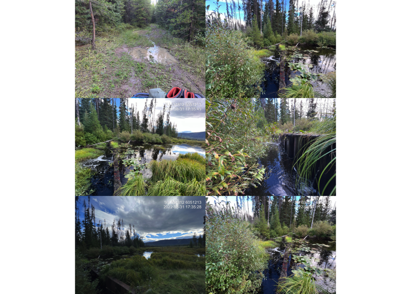
Figure 4.2: Photos of Dam 1f365462-063c-491e-9fb3-bfac004d9183 on Coffin Creek
#

model_url <- '<iframe src="https://www.mapsmadeeasy.com/maps/public/8e9c2ba6a3f845c2a3b1aa5047a4b39c" scrolling="no" title="Maps Made Easy" width="100%" height="600" frameBorder ="0"></iframe>'

knitr::asis_output(model_url)
my_photo = 'fig/pixel.png'
my_caption = paste0('Orthomosaic of Coffin Creek near Dam 1f365462-063c-491e-9fb3-bfac004d9183 To zoom press "shift" and scroll.')
knitr::include_graphics(my_photo, dpi = NA)Figure 4.3: Orthomosaic of Coffin Creek near Dam 1f365462-063c-491e-9fb3-bfac004d9183 To zoom press “shift” and scroll.
model_url <- '<iframe src="https://www.mapsmadeeasy.com/maps/public_3D/8e9c2ba6a3f845c2a3b1aa5047a4b39c" scrolling="no" title="Maps Made Easy" width="100%" height="600" frameBorder ="0"></iframe>'

knitr::asis_output(model_url)
my_photo = 'fig/pixel.png'
my_caption = paste0('3D model of habitat on Coffin Creek near Dam 1f365462-063c-491e-9fb3-bfac004d9183. To zoom press "shift" and scroll.')
knitr::include_graphics(my_photo, dpi = NA)Figure 4.4: 3D model of habitat on Coffin Creek near Dam 1f365462-063c-491e-9fb3-bfac004d9183. To zoom press “shift” and scroll.
4.3 Phase 1
Field assessments were conducted between August 29 2022 and September 10 2022 by Allan Irvine, R.P.Bio. and Mateo Winterscheidt, B.Sc., Tieasha Pierre, Vern Joseph, Dallas Nikal, Alexandria Nikal, Jesse Olson and Colin Morrison. A total of 9 Phase 1 assessments at sites not yet inventoried into the PSCIS system included 3 crossings considered “passable”, 0 crossings considered “potential” barriers and 3 crossings considered “barriers” according to threshold values based on culvert embedment, outlet drop, slope, diameter (relative to channel size) and length (MoE 2011a). Additionally, although all were considered fully passable, 3 crossings assessed were fords and ranked as “unknown” according to the provincial protocol. Georeferenced field maps are presented here and available for bulk download as Attachment 1. A summary of crossings assessed, a cost estimate for remediation and a priority ranking for follow up for Phase 1 sites is presented in Table 4.4. Detailed data with photos are presented in Appendix - Phase 1 Fish Passage Assessment Data and Photos.
“Barrier” and “Potential Barrier” rankings used in this project followed MoE (2011a) and reflect an assessment of passability for juvenile salmon or small resident rainbow trout at any flows potentially present throughout the year (Clarkin et al. 2005 ; Bell 1991; Thompson 2013). As noted in Bourne et al. (2011), with a detailed review of different criteria in Kemp and O’Hanley (2010), passability of barriers can be quantified in many different ways. Fish physiology (i.e. species, length, swim speeds) can make defining passability complex but with important implications for evaluating connectivity and prioritizing remediation candidates (Bourne et al. 2011; Shaw et al. 2016; Mahlum et al. 2014; Kemp and O’Hanley 2010). Washington Department of Fish & Wildlife (2009) present criteria for assigning passability scores to culverts that have already been assessed as barriers in coarser level assessments. These passability scores provide additional information to feed into decision making processes related to the prioritization of remediation site candidates and have potential for application in British Columbia.
 tab_cost_est_phase1 %>%
  select(`PSCIS ID`:`Cost Est ( $K)`) %>%
   fpr::fpr_kable(caption_text = 'Upstream habitat estimates and cost benefit analysis for Phase 1 assessments conducted on sites not yet inventoried in PSCIS. Steelhead network model (total length stream network <20% gradient).',
scroll = F)| PSCIS ID | External ID | Stream | Road | Result | Habitat value | Stream Width (m) | Priority | Fix | Cost Est ( $K) |
|---|---|---|---|---|---|---|---|---|---|
| 198115 | 2022091001 | Tributary to Waterfall Creek | 13 Avenue | Barrier | High | 2.8 | high | OBS | 2000 |
| 198116 | 2022091002 | Tributary to Waterfall Creek | Highway 16 | Barrier | High | 3.9 | high | OBS | 7500 |
| 198117 | 2022091003 | Tributary to Waterfall Creek | 9th Avenue | Barrier | High | 2.6 | high | OBS | 2000 |
4.4 Phase 2
During 2022 field assessments, habitat confirmation assessments were conducted at 7 sites in the Bulkley River watershed. A total of approximately 7km of stream was assessed, fish sampling utilizing electrofishing surveys were conducted at one stream. Georeferenced field maps are presented in here and available for bulk download as Attachment 1.
As collaborative decision making was ongoing at the time of reporting, site prioritization can be considered preliminary. In total, Three crossings were rated as high priorities for proceeding to design for replacement, 4 crossings were rated as moderate priorities, and 0 crossings were rated as low priorities. Results are summarized in Figure 4.1 and Tables 4.5 - 4.7 with raw habitat and fish sampling data included in digital format as Attachment 3. A summary of preliminary modelling results illustrating the quantity of chinook, coho and steelhead spawning and rearing habitat potentially available upstream of each crossing as estimated by measured/modelled channel width and upstream accessible stream length are presented in Figure 4.5. Detailed information for each site assessed with Phase 2 assessments (including maps) are presented within site specific appendices to this document.
table_phase2_overview <- function(dat, caption_text = '', font = font_set, scroll = TRUE){
  dat2 <- dat %>%
    kable(caption = caption_text, booktabs = T) %>%
    kableExtra::kable_styling(c("condensed"),
                              full_width = T,
                              font_size = font) %>%
    kableExtra::column_spec(column = c(9), width_min = '1.5in') %>%
    kableExtra::column_spec(column = c(5), width_max = '1in')

  if(identical(scroll,TRUE)){
    dat2 <- dat2 %>%
      kableExtra::scroll_box(width = "100%", height = "500px")
  }
  dat2
}

tab_overview %>%
  select(-Tenure) %>%
  table_phase2_overview(caption_text = 'Overview of habitat confirmation sites. Steelhead rearing model used for habitat estimates (total length of stream segments <7.5% gradient)',
scroll = gitbook_on)| PSCIS ID | Stream | Road | UTM (11U) | Fish Species | Habitat Gain (km) | Habitat Value | Priority | Comments |
|---|---|---|---|---|---|---|---|---|
| 57793 | Vallee Creek | Walcott Rd | 641460 6044049 | CAL,CT,LSU,RB | 3.4 | High | moderate | High value habitat with abundant undercut banks providing cover for resident fish. Some pockets of gravel present suitable for spawning. Large and small woody debris found throughout stream. 10:15:45 |
| 58067 | Gramophone Creek | Telkwa High Rd | 609736 6092880 | RB,ST | 3.4 | High | high | Small beaver dam ~500m upstream. Abundant cover. Approx. 50m of open residential area on right bank. Gravels suitable for spawning. 11:18 |
| 195943 | Stock Creek | Barrett Station Rd | 645434 6035035 | – | 0.7 | Medium | high | Good flow volume and complexity. Pockets of gravel suitable for resident rainbow spawning and potential coho. Channel constricted due to agricultural development on both sides of the stream. |
| 195944 | Stock Creek | Highway 16 | 646015 6035570 | – | 7.2 | Medium | moderate | Heavily impacted by cattle. Occasional pockets of gravel. Small rock drop of 65cm is located 365m upstream of the top end of the culvert. Massive culvert (170m long under 35m of fill). |
| 197653 | Perow Creek | Perow Loop Rd | 665520 6044200 | – | 7.4 | Low | moderate | No water until ~350m upstream, then abundant gravels and cobbles suitable for spawning with some deep pools and undercut banks. |
| 197974 | Watson Creek | Highway 16 | 680379 6040073 | CO, RB | 13.9 | Medium | moderate | Abundant gravels present for spawning. Lower 150-200m of stream heavily impacted by cattle. Beaver present in lower section. Numerous fry throughout. Some deep pools. Cattle impacts throughout. |
| 198116 | Waterfall Creek | Highway 16 | 590233 6123183 | CO, CT, RB, DV | 1.2 | High | high | Stream not mapped in freshwater atlas. Runs right through Hazelton. Watershed restoration plan in place by Skeena Conservation Coalition. Trap and truck coho operation. Station Creek downstream. |
fpr::fpr_table_cv_summary(dat = pscis_phase2) %>%
fpr::fpr_kable(caption_text = 'Summary of Phase 2 fish passage reassessments.', scroll = F)| PSCIS ID | Embedded | Outlet Drop (m) | Diameter (m) | SWR | Slope (%) | Length (m) | Final score | Barrier Result |
|---|---|---|---|---|---|---|---|---|
| 57793 | No | 0.10 | 3.0 | 1.6 | 2.0 | 20 | 24 | Barrier |
| 58067 | No | 0.49 | 2.2 | 3.0 | 0.3 | 16 | 29 | Barrier |
| 195943 | No | 1.10 | 2.0 | 1.5 | 1.5 | 14 | 31 | Barrier |
| 195944 | No | 1.50 | 1.8 | 1.4 | 3.5 | 99 | 42 | Barrier |
| 197653 | No | 0.30 | 2.3 | 1.9 | 1.5 | 28 | 34 | Barrier |
| 197974 | No | 1.00 | 0.9 | 3.8 | 3.5 | 26 | 39 | Barrier |
| 198116 | No | 0.00 | 1.5 | 2.6 | 2.5 | 27 | 24 | Barrier |
tab_cost_est_phase2_report %>%
  fpr::fpr_kable(caption_text = 'Cost benefit analysis for Phase 2 assessments. Steelhead rearing model used (total length of stream segments <7.5% gradient)',
scroll = gitbook_on)| PSCIS ID | Stream | Road | Result | Habitat value | Stream Width (m) | Fix | Cost Est (in $K) | Habitat Upstream (m) | Cost Benefit (m / $K) | Cost Benefit (m2 / $K) |
|---|---|---|---|---|---|---|---|---|---|---|
| 57793 | Vallee Creek | Walcott Road | Barrier | High | 4.1 | OBS | 2000 | 3440 | 1720.0 | 4042.0 |
| 58067 | Gramophone Creek | Telkwa high road | Barrier | High | 5.7 | OBS | 1150 | 3430 | 2982.6 | 9842.6 |
| 195943 | Stock Creek | Barrett Station Road | Barrier | Medium | 3.1 | OBS | 2000 | 740 | 370.0 | 555.0 |
| 195944 | Stock Creek | Highway 16 | Barrier | Medium | 4.2 | SS-CBS | 1500 | 7180 | 4786.7 | 6222.7 |
| 197653 | Perow Creek | Perow Loop Road | Barrier | Low | 3.2 | SS-CBS | 400 | 7390 | 18475.0 | 39721.2 |
| 197974 | Watson Creek | Highway 16 | Barrier | Medium | 3.4 | SS-CBS | 1500 | 13950 | 9300.0 | 15810.0 |
| 198116 | Tributary to Waterfall Creek | Highway 16 | Barrier | High | 3.7 | OBS | 7500 | 1200 | 160.0 | 312.0 |
tab_hab_summary %>%
  filter(Location %ilike% 'upstream') %>%
  select(-Location) %>%
  rename(`PSCIS ID` = Site, `Length surveyed upstream (m)` = `Length Surveyed (m)`) %>%
fpr::fpr_kable(caption_text = 'Summary of Phase 2 habitat confirmation details.', scroll = F)| PSCIS ID | Length surveyed upstream (m) | Channel Width (m) | Wetted Width (m) | Pool Depth (m) | Gradient (%) | Total Cover | Habitat Value |
|---|---|---|---|---|---|---|---|
| 57793 | 600 | 4.1 | 2.0 | – | 2.0 | abundant | high |
| 58067 | 600 | 5.7 | 4.0 | 0.3 | 3.0 | moderate | high |
| 195943 | 330 | 3.1 | 1.8 | 0.3 | 2.1 | abundant | medium |
| 195944 | 640 | 4.2 | 1.8 | 0.3 | 2.0 | moderate | medium |
| 197653 | 500 | 3.2 | 1.9 | 0.4 | 3.0 | moderate | medium |
| 197653 | 150 | 4.7 | 2.4 | 0.6 | 3.7 | moderate | medium |
| 197974 | 600 | 3.4 | 1.8 | 0.5 | 1.8 | moderate | medium |
| 198116 | 1200 | 3.7 | 3.5 | 0.3 | 1.5 | abundant | high |
fpr::fpr_table_wshd_sum() %>%
  fpr::fpr_kable(caption_text = paste0('Summary of watershed area statistics upstream of Phase 2 crossings.'),
footnote_text = 'Elev P60 = Elevation at which 60% of the watershed area is above', scroll = F)| Site | Area Km | Elev Site | Elev Min | Elev Max | Elev Median | Elev P60 | Aspect |
|---|---|---|---|---|---|---|---|
| 57793 | 21.7 | 617 | 646 | 1370 | 847 | 828 | SW |
| 58067 | 33.3 | 459 | – | 1480 | 1043 | 951 | WSW |
| 195943 | 14.3 | 636 | 681 | 1274 | 923 | 892 | SW |
| 195944 | 14.3 | 689 | 681 | 1274 | 923 | 892 | SW |
| 197653 | 16.4 | 649 | 810 | 1412 | 991 | 970 | SSE |
| 197974 | 17.9 | 731 | 771 | 1415 | 950 | 922 | SSW |
| * Elev P60 = Elevation at which 60% of the watershed area is above |
bcfp_xref_plot <- xref_bcfishpass_names %>%
  filter(!is.na(id_join) &
           !bcfishpass %ilike% 'below' &
           !bcfishpass %ilike% 'all' &
           !bcfishpass %ilike% '_ha' &
           (bcfishpass %ilike% 'rearing' |
              bcfishpass %ilike% 'spawning'))

bcfishpass_phase2_plot_prep <- bcfishpass %>%
  mutate(across(where(is.numeric), round, 1)) %>%
    filter(stream_crossing_id %in% (pscis_phase2 %>% pull(pscis_crossing_id))) %>%
  select(stream_crossing_id, all_of(bcfp_xref_plot$bcfishpass)) %>%
  # filter(stream_crossing_id != 197665) %>%
  mutate(stream_crossing_id = as.factor(stream_crossing_id)) %>%
  pivot_longer(cols = ch_spawning_km:st_rearing_km)  %>%
  filter(value > 0.0 &
           !is.na(value)
         , !name %ilike% 'sk'
         ) %>%
  mutate(
    # name = stringr::str_replace_all(name, '_belowupstrbarriers_km', ''),
         name = stringr::str_replace_all(name, '_rearing', ' rearing'),
         name = stringr::str_replace_all(name, '_spawning', ' spawning'))
    # rename('Habitat type' = name,
    #        "Habitat (km)" = value)


 bcfishpass_phase2_plot_prep %>%
  ggplot(aes(x = stream_crossing_id, y = value)) +
  geom_bar(stat = "identity")+
  facet_wrap(~name, ncol = 2)+
  ggdark::dark_theme_bw(base_size = 11)+
   theme(axis.text.x=element_text(angle=90, hjust=1, vjust=0.5)) +
  labs(x = "Site", y = "Modelled habitat (km)")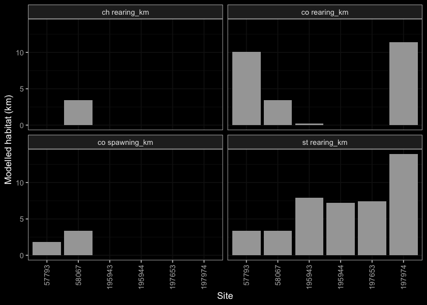
Figure 4.5: Summary of potential habitat upstream of habitat confirmation assessment sites estimated based on modelled channel width and upstream channel length.
4.4.1 Fish Sampling
Fish sampling was conducted at 12 sites in Gramaphone Creek (6 sites upstream and 6 sites downstream of Telkwa High Road) with a total of 50 rainbow trout captured. Fork length data was used to delineate salmonids based on life stages: fry (0 to 65mm), parr (>65 to 115mm), juvenile (>115mm to 145mm) and adult (>145mm) by visually assessing the histograms presented in Figure 4.6. A summary of sites assessed are included in Table 4.11 and raw data is provided in Attachment 3. A summary of density results for all life stages combined of select species is also presented in Figure 4.7. Results are presented in greater detail within individual habitat confirmation site appendices.
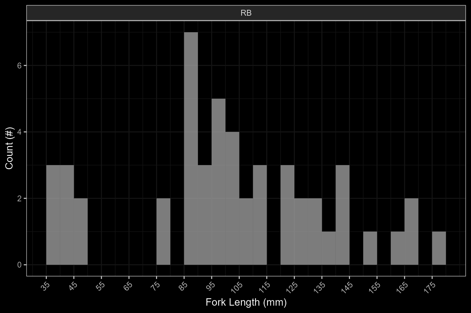
Figure 4.6: Histograms of fish lengths by species. Fish captured by electrofishing during habitat confirmation assessments.
tab_fish_sites_sum %>%
fpr::fpr_kable(caption_text = 'Summary of electrofishing sites.', scroll = F)| site | passes | ef_length_m | ef_width_m | area_m2 | enclosure |
|---|---|---|---|---|---|
| 58067_ds_ef1 | 1 | 15.9 | 3.3 | 52.5 | open |
| 58067_ds_ef2 | 1 | 24.0 | 3.6 | 86.4 | open |
| 58067_ds_ef3 | 1 | 25.2 | 3.5 | 88.2 | open |
| 58067_ds_ef4 | 1 | 32.2 | 3.4 | 109.5 | open |
| 58067_ds_ef5 | 1 | 13.0 | 2.6 | 33.8 | open |
| 58067_ds_ef6 | 1 | 7.7 | 5.6 | 43.1 | open |
| 58067_us_ef1 | 1 | 8.6 | 3.4 | 29.2 | open |
| 58067_us_ef2 | 1 | 19.8 | 2.8 | 55.4 | open |
| 58067_us_ef3 | 1 | 25.2 | 3.5 | 88.2 | open |
| 58067_us_ef4 | 1 | 32.2 | 2.8 | 90.2 | open |
| 58067_us_ef5 | 1 | 13.0 | 3.1 | 40.3 | open |
| 58067_us_ef6 | 1 | 6.0 | 4.0 | 24.0 | open |
plot_fish_box_all <-  fish_abund %>% #tab_fish_density_prep
    filter(
      !species_code %in% c('MW', 'SU', 'NFC', 'CT', 'LSU')
    ) %>%
    ggplot(., aes(x = location, y =density_100m2)) +
    geom_boxplot()+
    facet_grid(site ~ species_code, scales ="fixed", #life_stage
               as.table = T)+
    # theme_bw()+
    theme(legend.position = "none", axis.title.x=element_blank()) +
    geom_dotplot(binaxis='y', stackdir='center', dotsize=1)+
    ylab(expression(Density ~ (Fish/100 ~  m^2))) +
    ggdark::dark_theme_bw()

plot_fish_box_all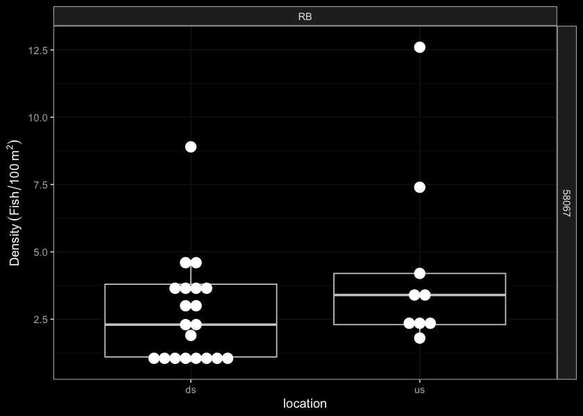
Figure 4.7: Boxplots of densities (fish/100m2) of fish captured by electrofishing during habitat confirmation assessments.
4.5 Phase 3
Engineering designs have been completed for replacement of PSCIS crossing 58159 on McDowell Creek (Irvine 2021) with a clear-span bridge and for removal of the collapsed bridge (PSCIS crossing 197912) on Robert Hatch Creek. Designs for McDowell and Robert Hatch were procured by SERNbc and Canadian Wildlife Federation respectively. At the time of reporting, the Ministry of Transportation and Infrastructure, in collaboration with Canadian Wildlife Federation was in the process of procuring designs for remediation of fish passage at three sites documented in Irvine (2021) including PSCIS 123445 on Tyhee Creek, PSCIS 124500 on Helps Creek and PSCIS 197640 on a tributary to Buck Creek. Additionally, the Ministry of Transportation and Infrastructure were procuring a design for PSCIS crossing 124420 on Station Creek (also know as Mission Creek) near New Hazleton (pers. comm. Sean Wong, Environmental Programs, MoTi).