4 Results and Discussion
Results of Planning, Phase 1 and Phase 2 assessments are summarized in Figure 4.1 with additional details provided in sections below.
##make colors for the priorities
pal <-
   colorFactor(palette = c("red", "yellow", "grey", "black"),
               levels = c("high", "moderate", "low", "no fix"))

pal_phase1 <-
   colorFactor(palette = c("red", "yellow", "grey", "black"),
               levels = c("high", "moderate", "low", NA))

tab_map_phase2 <- tab_map %>% filter(source %like% 'phase2')
#https://stackoverflow.com/questions/61026700/bring-a-group-of-markers-to-front-in-leaflet
# marker_options <- markerOptions(
#   zIndexOffset = 1000)
tracks <- sf::read_sf("./data/habitat_confirmation_tracks.gpx", layer = "tracks")
  # filter(!pscis_crossing_id %in% c(62423, 62426, 50181, 50159)) ##these ones are not correct - fix later

wshd_study_areas <- sf::read_sf('data/fishpass_mapping/fishpass_mapping.gpkg', layer = 'wshd_study_areas')
  # st_transform(crs = 4326)
# photo_metadata <- readr::read_csv(file = 'data/photo_metadata.csv')


map <- leaflet(height=500, width=780) %>%
  # leaflet() %>%
  addTiles()  %>%
  # leafem::addMouseCoordinates(proj4 = 26911) %>% ##can't seem to get it to render utms yet
  # addProviderTiles(providers$"Esri.DeLorme") %>%
  addProviderTiles("Esri.WorldTopoMap", group = "Topo") %>%
  addProviderTiles("Esri.WorldImagery", group = "ESRI Aerial") %>%

  addPolygons(data = wshd_study_areas %>%
                filter(watershed_group_code == 'ELKR'),
              color = "#C39D50",
              weight = 1,
              smoothFactor = 0.5,
              opacity = 1.0,
              fillOpacity = 0.2,
              fillColor = "#C39D50",
              label = 'Elk River Watershed Group') %>%
  addPolygons(data = wshds, color = "#0859C6", weight = 1, smoothFactor = 0.5,
    opacity = 1.0, fillOpacity = 0.25,
    fillColor = "#00DBFF",
    label = wshds$stream_crossing_id,
    popup = leafpop::popupTable(x = select(wshds %>% st_set_geometry(NULL),
                                           Site = stream_crossing_id,
                                           elev_min:area_km),
                                feature.id = F,
                                row.numbers = F),
    group = "Phase 2") %>%
  # addPolygons(data = wshd_study_areas %>% filter(watershed_group_code == 'MORR'), color = "#C39D50", weight = 1, smoothFactor = 0.5,
  #   opacity = 1.0, fillOpacity = 0,
  #   fillColor = "#C39D50", label = 'Morice River') %>%
  # addPolylines(data=forest_tenure_road_lines,  opacity=1, color = '#ff7f00',
  #              fillOpacity = 0.75, weight=2) %>%
    addLegend(
    position = "topright",
    colors = c("red", "yellow", "grey", "black"),
    labels = c("High", "Moderate", "Low", 'No fix'), opacity = 1,
    title = "Fish Passage Priorities",
  ) %>%
    # addCircleMarkers(
    # data=tab_plan_sf,
    # label = tab_plan_sf$Comments,
    # labelOptions = labelOptions(noHide = F, textOnly = F),
    # popup = leafpop::popupTable(x = tab_plan_sf %>% st_drop_geometry(),
    #                             feature.id = F,
    #                             row.numbers = F),
    # radius = 9,
    # fillColor = ~pal_phase1(tab_plan_sf$Priority),
    # color= "#ffffff",
    # stroke = TRUE,
    # fillOpacity = 1.0,
    # weight = 2,
    # opacity = 1.0,
    # group = "Planning") %>%

    addCircleMarkers(data=tab_map %>% filter(source %like% 'phase1' | source %like% 'pscis_reassessments'),
    label = tab_map %>% filter(source %like% 'phase1' | source %like% 'pscis_reassessments') %>% pull(pscis_crossing_id),
    # label = tab_map$pscis_crossing_id,
    labelOptions = labelOptions(noHide = F, textOnly = TRUE),
    popup = leafpop::popupTable(x = select((tab_map %>% st_set_geometry(NULL) %>% filter(source %like% 'phase1' | source %like% 'pscis_reassessments')),
                                           Site = pscis_crossing_id,
                                           Priority = priority_phase1,
                                           Stream = stream_name,
                                           Road = road_name,
                                           `Habitat value`= habitat_value,
                                           `Barrier Result` = barrier_result,
                                           `Culvert data` = data_link,
                                           `Culvert photos` = photo_link),
                                feature.id = F,
                                row.numbers = F),
    radius = 9,
    fillColor = ~pal_phase1(priority_phase1),
    color= "#ffffff",
    stroke = TRUE,
    fillOpacity = 1.0,
    weight = 2,
    opacity = 1.0,
    group = "Phase 1"
    ) %>%

    addPolylines(data=tracks,
                 opacity=0.75, color = '#e216c4',
               fillOpacity = 0.75, weight=5, group = "Phase 2") %>%
  addAwesomeMarkers(
    lng = photo_metadata$gps_longitude,
    lat = photo_metadata$gps_latitude,
    popup = leafpop::popupImage(photo_metadata$url, src = "remote"),
    clusterOptions = markerClusterOptions(),
    group = "Phase 2") %>%

    addCircleMarkers(
    data=tab_hab_map,
    label = tab_hab_map$pscis_crossing_id,
    labelOptions = labelOptions(noHide = T, textOnly = TRUE),
    popup = leafpop::popupTable(x = select((tab_hab_map %>% st_set_geometry(NULL)),
                                           Site = pscis_crossing_id,
                                           Priority = priority,
                                           Stream = stream_name,
                                           Road = road_name,
                                           `Habitat (m)`= upstream_habitat_length_m,
                                           Comments = comments,
                                           `Culvert data` = data_link,
                                           `Culvert photos` = photo_link,
                                           `Model data` = model_link),
                                feature.id = F,
                                row.numbers = F),
    radius = 9,
    fillColor = ~pal(priority),
    color= "#ffffff",
    stroke = TRUE,
    fillOpacity = 1.0,
    weight = 2,
    opacity = 1.0,
    group = "Phase 2"
    ) %>%
  #     # addScaleBar(position = 'bottomleft', options = scaleBarOptions(imperial = FALSE)) %>%
  addLayersControl(
    baseGroups = c(
      "Esri.DeLorme",
      "ESRI Aerial"),
    overlayGroups = c("Phase 1",
                      "Phase 2"),
    options = layersControlOptions(collapsed = F)) %>%
  leaflet.extras::addFullscreenControl() %>%
  addMiniMap(tiles = providers$"Esri.NatGeoWorldMap",
             zoomLevelOffset = -6, width = 100, height = 100)

map %>%
  hideGroup(c("Phase 1")) %>%
  setView(lat = st_centroid(wshd_study_areas) %>% mutate(lat = sf::st_coordinates(.)[,2]) %>% pull(lat),
          lng = st_centroid(wshd_study_areas) %>% mutate(lng = sf::st_coordinates(.)[,1])%>% pull(lng),
          zoom = 8)
Figure 4.1: Map of fish passage and habitat confirmation results
 # mutate(long = sf::st_coordinates(.)[,1],
 #        lat = sf::st_coordinates(.)[,2])
4.1 Phase 1
Field assessments were conducted between July 27 2021 and November 03 2021 by Allan Irvine, R.P.Bio., Kyle Prince, P.Biol., Stevie Syer, Environmental Technician, Rafael Acosta Lugo, M.Sc., Environmental Technician and Brody Klenk, Environmental Technician. A total of 89 Phase 1 assessments were conducted at 89 sites with 19 crossings considered “passable”, 1 crossing considered “potential” barriers and 31 crossing considered “barriers” according to threshold values based on culvert embedment, outlet drop, slope, diameter (relative to channel size) and length (MoE 2011a). Additionally, although all were considered fully passable, 38 crossings assessed were fords. Georeferenced field maps are presented here and available for bulk download as Attachment 1. A summary of crossings assessed, a cost benefit analysis and priority ranking for follow up for Phase 1 sites with barrier status of “barrier” or “potential barrier” according to provincial metric are presented in Table 4.1. Detailed data with photos are presented in Appendix - Phase 1 Fish Passage Assessment Data and Photos.
“Barrier” and “Potential Barrier” rankings used in this project followed MoE (2011a) and reflect an assessment of passability for juvenile salmon or small resident rainbow trout at any flows potentially present throughout the year (Clarkin et al. 2005 ; Bell 1991; Thompson 2013). As noted in Bourne et al. (2011), with a detailed review of different criteria in Kemp and O’Hanley (2010), passability of barriers can be quantified in many different ways. Fish physiology (i.e. species, length, swim speeds) can make defining passability complex but with important implications for evaluating connectivity and prioritizing remediation candidates (Bourne et al. 2011; Shaw et al. 2016; Mahlum et al. 2014; Kemp and O’Hanley 2010). Washington Department of Fish & Wildlife (2009) present criteria for assigning passability scores to culverts that have already been assessed as barriers in coarser level assessments. These passability scores provide additional information to feed into decision making processes related to the prioritization of remediation site candidates and have potential for application in British Columbia.
#`r if(identical(gitbook_on, FALSE)){knitr::asis_output("<br>")}`
if(gitbook_on){
  tab_cost_est_phase1 %>%
  my_kable_scroll(caption_text = 'Upstream habitat estimates and cost benefit analysis for Phase 1 assessments with barrier status of "barrier" or "potential barrier" according to provincial metric.  ')
} else tab_cost_est_phase1 %>%
my_kable(caption_text = 'Upstream habitat estimates and cost benefit analysis for Phase 1 assessments with barrier status of "barrier" or "potential barrier" according to provincial metric.')| PSCIS ID | External ID | Stream | Road | Result | Habitat value | Stream Width (m) | Priority | Fix | Cost Est ( $K) | Habitat Upstream (km) | Cost Benefit (m / $K) | Cost Benefit (m2 / $K) |
|---|---|---|---|---|---|---|---|---|---|---|---|---|
| 50075 | – | Tributary to Flathead FSR | Commerce FSR | Barrier | Low | 1.90 | low | SS-CBS | 40 | 1.97 | 49.2 | 46.8 |
| 50084 | – | Tributary to Flathead River | Flathead FSR | Potential | Medium | 2.40 | low | OBS | 240 | 2.26 | 9.4 | 11.3 |
| 50085 | – | Tributary to Couldrey Creek | Flathead FSR | Barrier | Low | 2.40 | low | OBS | 240 | 4.05 | 16.9 | 20.2 |
| 50091 | – | Tributary to Calder Creek | Spur | Barrier | Low | 1.50 | low | SS-CBS | 40 | 2.31 | 57.8 | 43.3 |
| 197835 | 4600088 | Hosmer Creek | Stephenson Road | Barrier | Medium | 4.10 | mod | OBS | 1920 | – | – | – |
| 197833 | 4600129 | Hosmer Creek | Highway 3 | Barrier | Medium | 3.00 | mod | OBS | 7200 | – | – | – |
| 197863 | 4600761 | Tributary to Lizard Creek | Unnamed | Barrier | Low | 2.00 | low | OBS | 240 | – | – | – |
| 197827 | 4600762 | Fording River | FRO Coal Haul | Barrier | High | 16.00 | high | OBS | 660 | – | – | – |
| 197866 | 4600992 | Hosmer Creek | Unnamed | Barrier | High | 4.10 | high | OBS | 240 | – | – | – |
| 197796 | 4601984 | Tributary to Lodgepole Creek | Spur | Barrier | Low | 3.80 | low | OBS | 240 | – | – | – |
| 197825 | 4604677 | Henretta Creek | – | Barrier | High | 12.00 | high | OBS | 360 | – | – | – |
| 197851 | 4605462 | Tributary to Flathead River | Kishinea FSR | Barrier | Low | 1.20 | low | SS-CBS | 40 | – | – | – |
| 197843 | 4605502 | Tributary to Bighorn Creek | Cabin FSR | Barrier | Medium | 1.80 | mod | SS-CBS | 40 | – | – | – |
| 197842 | 4605504 | Tributary to Bighorn Creek | Cabin FSR | Barrier | Medium | 2.10 | mod | OBS | 240 | – | – | – |
| 197844 | 4605514 | Tributary to Bighorn Creek | Cabin FSR | Barrier | Medium | 2.20 | mod | OBS | 240 | – | – | – |
| 197798 | 4605518 | Tributary to Bighorn Creek | Cabin FSR | Barrier | Low | 1.00 | low | SS-CBS | 40 | – | – | – |
| 197799 | 4605522 | Tributary to Bighorn Creek | Cabin FSR | Barrier | Low | 1.30 | low | SS-CBS | 40 | – | – | – |
| 197800 | 4605525 | Tributary to Bighorn Creek | Cabin FSR | Barrier | Medium | 1.90 | mod | SS-CBS | 40 | – | – | – |
| 197845 | 4605531 | Tributary to Bighorn Creek | Cabin FSR | Barrier | Low | 2.50 | low | OBS | 240 | – | – | – |
| 197802 | 4605540 | Tributary to Bighorn Creek | Cabin FSR | Barrier | Low | 1.60 | low | SS-CBS | 40 | – | – | – |
| 197850 | 4605584 | Tributary to Sage Creek | Flathead-Nettie FSR | Barrier | Low | 2.10 | low | OBS | 240 | – | – | – |
| 197849 | 4605585 | Tributary to Sage Creek | Flathead-Nettie FSR | Barrier | Low | 1.70 | low | SS-CBS | 40 | – | – | – |
| 197865 | 4605652 | Tributary to Elk River | Elk River Main FSR | Barrier | Low | 1.00 | low | SS-CBS | 40 | – | – | – |
| 197828 | 4605671 | Tributary to Elk River | Elk FSR | Barrier | Low | 1.30 | low | SS-CBS | 40 | – | – | – |
| 197829 | 4605698 | Tributary to Elk River | Elk FSR | Barrier | Low | 0.95 | low | SS-CBS | 40 | – | – | – |
| 197830 | 4605731 | Tributary to Elk River | Elk FSR | Barrier | Medium | 2.00 | mod | OBS | 240 | – | – | – |
| 197783 | 4605937 | Tributary to Wigwam River | Wigwam FSR | Barrier | Low | 0.60 | low | SS-CBS | 40 | – | – | – |
| 197817 | 4605995 | Tributary to Weigert Creek | Weigert FSR | Barrier | Low | 2.40 | low | OBS | 240 | – | – | – |
| 197785 | 4606129 | Tributary to Wigwam River | – | Barrier | Low | 0.00 | low | SS-CBS | 40 | – | – | – |
| 197793 | 4606347 | Tributary to Bean Creek | Lodgepole FSR | Barrier | Low | 5.30 | low | OBS | 240 | – | – | – |
| 197787 | 4606370 | Lodgepole Creek | Harvey FSR | Potential | Medium | 3.26 | low | OBS | 240 | – | – | – |
| 197786 | 4606398 | Lodgepole Creek | Harvey FSR | Barrier | Medium | 2.00 | mod | OBS | 240 | – | – | – |
| 197809 | 4606597 | Tributary to Flathead River | Commerce FSR | Barrier | Low | 0.90 | low | SS-CBS | 40 | – | – | – |
| 197834 | 4606711 | Hosmer Creek | CP Railway | Barrier | High | 3.90 | high | OBS | 7200 | – | – | – |
| 197855 | 24740603 | Tributary to Calder Creek | Spur 1000 | Barrier | Low | 0.80 | low | SS-CBS | 40 | – | – | – |
| 197864 | 2021101302 | Tributary to Lizard Creek | Unnamed | Barrier | Low | 0.50 | low | SS-CBS | 40 | – | – | – |
4.2 Dam Assessments
Three historic dam locations were assessed for fish passage including sites on Hartley Creek, Boivin Creek, and Harmer Creek. Results are presented in Table 4.2
tab_dams_raw %>%
  select(-utm_zone) %>%
  arrange(id) %>%
  purrr::set_names(nm = c('Site', 'Stream', 'Easting', 'Northing', 'Mapsheet', 'Barrier', 'Notes')) %>%
  my_kable(caption_text = 'Results from fish passability assessments at dams.',
footnote_text = 'UTM Zone 11')| Site | Stream | Easting | Northing | Mapsheet | Barrier | Notes |
|---|---|---|---|---|---|---|
| 197542 | Hartley Creek | 643537 | 5490723 | 082G.113 | T | Two small dams (30cm and 40cm high) located just upstream (7m and 20m) of Dicken Road. Likely easily passable by adult WCT but barrier to fry and small juveniles. If culvert replaced these could potentially be fixed at the same time. |
| 1100000129 | Boivin Creek | 647275 | 5541987 | 082J.103 | F | Remnant dam not located in main channel. |
| 1100002016 | Harmer Creek | 657051 | 5522119 | 082G.123 | T | Large dam (15m high at 55% grade) located in main channel. No fish ladder. |
| * UTM Zone 11 |
my_site = 197542
my_photo1 = pull_photo_by_str(str_to_pull = '_1_')

my_caption1 = paste0('Small dam ~7m upstream of PSCIS crossing ', my_site, ' on Hartley Creek.')grid::grid.raster(get_img(photo = my_photo1))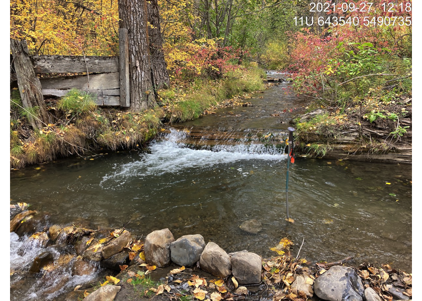
Figure 4.2: Small dam ~7m upstream of PSCIS crossing 197542 on Hartley Creek.
my_photo2 = pull_photo_by_str(str_to_pull = '_2_')

my_caption2 = paste0('Small dam ~20m upstream of PSCIS crossing ', my_site, ' on Hartley Creek.')grid::grid.raster(get_img(photo = my_photo2))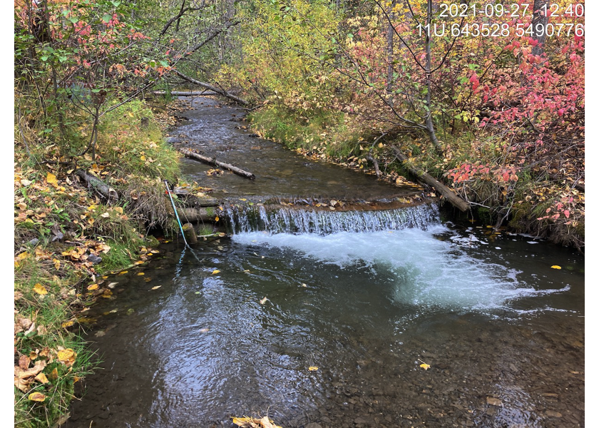
Figure 4.3: Small dam ~20m upstream of PSCIS crossing 197542 on Hartley Creek.
my_caption <- paste0('Left: ', my_caption1, ' Right: ', my_caption2)

knitr::include_graphics(get_img_path(photo = my_photo1))
knitr::include_graphics("fig/pixel.png")
knitr::include_graphics(get_img_path(photo = my_photo2))
my_site = 1063 #old id
my_photo1 = pull_photo_by_str(str_to_pull = '_1_')
my_caption1 = paste0('Teck Coal Limited dam (15m high and 55% gradient) on Harmer Creek.')grid::grid.raster(get_img(photo = my_photo1))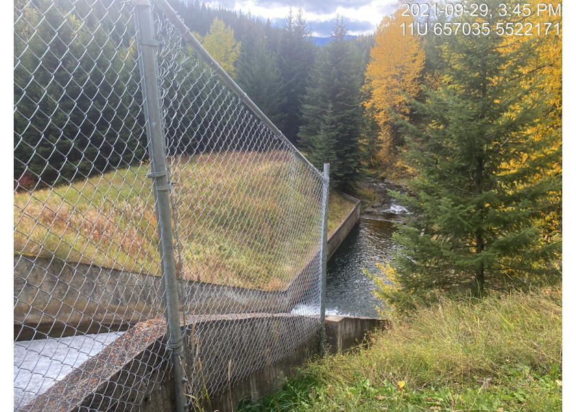
Figure 4.4: Teck Coal Limited dam (15m high and 55% gradient) on Harmer Creek.
my_site2 = 2606
my_photo2 = pull_photo_by_str(site_id = my_site2,str_to_pull = '_1_')

my_caption2 = paste0('Historic dam structure adjacent to Boivin Creek.')grid::grid.raster(get_img(site = my_site2, photo = my_photo2))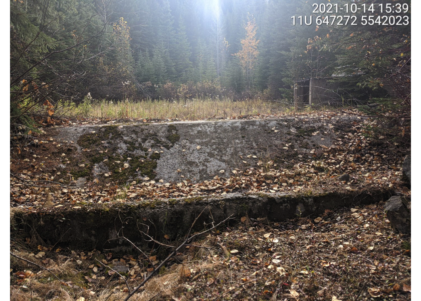
Figure 4.5: Historic dam structure adjacent to Boivin Creek.
my_caption <- paste0('Left: ', my_caption1, ' Right: ', my_caption2)

knitr::include_graphics(get_img_path(photo = my_photo1))
knitr::include_graphics("fig/pixel.png")
knitr::include_graphics(get_img_path(site = my_site2, photo = my_photo2))
4.3 Phase 2
During 2021 field assessments, habitat confirmation assessments were conducted at 15 sites in the Elk River watershed group with a total of approximately 12km of stream assessed. Georeferenced field maps are presented here and available for bulk download as Attachment 1.
As collaborative decision making was ongoing at the time of reporting, site prioritization can be considered preliminary. Five crossings were rated as high priorities for proceeding to design for replacement, 7 crossings were rated as moderate priorities, and 3 crossings were rated as low priorities. Results are summarized in Figure 4.1 and Table 4.3) with raw habitat assessment data included in digital format as Attachment 3. A summary of watershed statistics from derived watershed areas and preliminary modeling results illustrating the quantities of westslope cutthrout trout spawning and rearing habitat potentially available upstream of each crossing as estimated by upstream accessible stream length are presented in Table 4.7 and Figure 4.6. Only summary tables and raw data is provided for surveys conducted within the Flathead River sub-basin (Parker Creek, Morris Creek, Fuel Creek and Kisoo Creek) with detailed reporting potentially provided in the future under separate cover. Detailed information for each site assessed with Phase 2 assessments (including georeferenced maps) on streams that drain into the Elk River are presented within site specific appendices to this document.
#`r if(gitbook_on){knitr::asis_output("<br>")} else knitr::asis_output("<br><br><br><br><br><br><br><br><br><br><br><br><br><br><br><br><br><br><br><br><br><br><br><br><br><br><br><br><br><br><br>")`
if(gitbook_on){
tab_overview %>%
  select(-Tenure) %>%
  my_tab_overview_scroll(caption_text = 'Overview of habitat confirmation sites.')
} else tab_overview %>%
  select(-Tenure) %>%
my_kable(caption_text = 'Overview of habitat confirmation sites.')| PSCIS ID | Stream | Road | UTM (11U) | Fish Species | Habitat Gain (km) | Habitat Value | Priority | Comments |
|---|---|---|---|---|---|---|---|---|
| 50061 | Fuel Creek | Harvey FSR | 667651 5459223 | WCT | 2.0 | Medium | moderate | Signs of extremely high flows with large islands and dry side channels. First 200m were dry. Old road sluffing at times and for ~50m was right beside creek eliminating riparian veg. Ranked as high priority for follow up in Irvine 2021. |
| 50063 | Kisoo Creek | Harvey FSR | 668961 5458806 | – | 1.3 | Medium | moderate | Fairly steep system with frequent pockets of gravels available for spawning. Cold high elevation system with good flow and abundant undercut banks. |
| 50067 | Parker Creek | Flathead FSR | 679597 5453756 | WCT | 6.0 | High | high | Parker creek remnant channel similar to upstream size and depth with no water. Channel relocation related to Flathead FSR with several large volume beaver controlled wetland areas upstream in historic channel. Aerial survey conducted. Needs to be fixed in conjunction with mocelled crossing 4606967 upstream (currently no structure there). Great opportunity for restoration. |
| 61504 | Coal Creek | Coal Creek Road | 645313 5483687 | WCT, BT | 14.5 | – | high | Issue is not structure but debris in channel producing small drop/cascade from 20 - 60cmin height. Some deep pools up to ~1.8m available for overwintering westslope cutthroat trout adults. Some pockets for spawning, large system with low gradient. Mature ACT riparian area with intermittent large woody debris structures throughout. |
| 62122 | Morris Creek | Flathead FSR | 676913 5459598 | – | 3.0 | Medium | moderate | Good flow, frequent pockets of gravels present suitable for westslope cutthroat trout spawning. Unlicensed dam located upstream of road ~100m. Main flow of stream is north fork with small amount of flow from southern forks. Erroneosly ranked as low priority for follow up in Irvine 2021 due to incorrect mapping of mainstem of channel. |
| 62181 | Dry Creek | CP Railway | 656409 5544755 | WCT | 4.3 | Medium | high | Line Creek Operations Local Aquatic Effects Monitoring Program underway here with plan for fish passage remediation part of Teck’s Tributary management Plan. Flagging from FHAP conducted by other crews. High value habitat due to flow and size, occasional pockets of gravel and intermittent pools. |
| 62182 | Dry Creek | Fording Highway | 656390 5544771 | WCT | 0.0 | Medium | high | FHAP conducted here by other crews. High value habitat due to flow and size, occasional pockets of gravel and intermittent pools. |
| 62505 | Tributary to Lizard Creek | Mt. Fernie Park Road | 636942 5483777 | – | 0.7 | Medium | moderate | Occasional pools present suitable for juvenile westslope cutthroat trout overwintering. Frequent pockets of gravel present suitable for spawning. Good flow. Fairly steep system with intermittent small woody debris / root drops between 0.5 and 1m. |
| 197786 | Lodgepole Creek | Harvey FSR | 665796 5462152 | – | 0.6 | Medium | moderate | Small stream with good flow. Abundant gravels suitable for spawning throughout the first ~300m then pockets throughout. Large waterfall >30m at top end of site ~540m u/s of culvert. Some shallow pools present intermittently created by large woody debris. |
| 197787 | Lodgepole Creek | Harvey FSR | 664905 5462562 | WCT | 1.1 | Medium | moderate | Drains out of Lodgepole Lake. Beaver Dam (1.2m) at lake. Abundant gravels suitable for spawning throughout. Stream primarily had low complexity due to the primarily straight riffle type habitat. Some shallow pools and large woody debris present. |
| 197793 | Bean Creek | Lodgepole FSR | 650415 5463819 | – | 1.8 | Low | low | Dry stream, no water. Has very large channel and shows evidence of extensive scour and large volumes of water but completely dry. |
| 197796 | Tributary to Lodgepole Creek | Spur | 654302 5458678 | – | 0.1 | Low | low | 2.3m high rock falls at ~60m upstream is permanent barrier to upstream migration. |
| 197844 | Tributary to Bighorn Creek | Cabin FSR | 657920 5452802 | – | 0.8 | Medium | moderate | Sections getting steep (up to 12.5%) with periodic deep pools under embedded / functional large woody debris. Likely barrier ( 1.1m high rock) located at top of area surveyed 840m upstream of the FSR. Frequent cascading into pools. Confined at times. |
fpr_make_tab_cv(dat = pscis_phase2) %>%
my_kable(caption_text = 'Summary of Phase 2 fish passage reassessments.')| PSCIS ID | Embedded | Outlet Drop (m) | Diameter (m) | SWR | Slope (%) | Length (m) | Final score | Barrier Result |
|---|---|---|---|---|---|---|---|---|
| 50061 | Yes | 0.00 | 0.9 | 3.2 | 3.0 | 14 | 16 | Potential |
| 50063 | No | 0.65 | 1.2 | 2.3 | 5.0 | 45 | 42 | Barrier |
| 50067 | No | 0.00 | 0.6 | 8.7 | 3.0 | 11 | 26 | Barrier |
| 61504 | – | – | 24.0 | 0.0 | – | 4 | 0 | Passable |
| 62122 | No | 0.00 | 0.9 | 1.7 | 4.5 | 10 | 26 | Barrier |
| 62181 | Yes | 0.00 | 1.8 | 2.1 | 2.6 | 17 | 19 | Potential |
| 62182 | No | 0.00 | 1.8 | 2.1 | 3.6 | 24 | 29 | Barrier |
| 62505 | No | 0.25 | 0.9 | 3.2 | 5.0 | 10 | 31 | Barrier |
| 197786 | No | 0.00 | 1.2 | 1.7 | 1.7 | 10 | 21 | Barrier |
| 197787 | No | 0.00 | 2.0 | 1.6 | 0.5 | 18 | 19 | Potential |
| 197793 | No | 0.00 | 1.5 | 3.5 | 2.5 | 14 | 21 | Barrier |
| 197796 | No | 0.60 | 1.6 | 2.4 | 5.0 | 14 | 36 | Barrier |
| 197844 | No | 1.20 | 1.2 | 1.8 | 5.0 | 12 | 36 | Barrier |
tab_cost_est_phase2_report %>%
my_kable(caption_text = 'Cost benefit analysis for Phase 2 assessments.')| PSCIS ID | Stream | Road | Result | Habitat value | Stream Width (m) | Fix | Cost Est (in $K) | Habitat Upstream (m) | Cost Benefit (m / $K) | Cost Benefit (m2 / $K) |
|---|---|---|---|---|---|---|---|---|---|---|
| 50061 | Fuel Creek | Harvey FSR | Potential | Medium | 3.1 | OBS | 240 | 2000 | 8.3 | 25.8 |
| 50063 | Kisoo Creek | Harvey FSR | Barrier | Medium | 2.8 | SS-CBS | 80 | 1280 | 16.0 | 44.8 |
| 50067 | Parker Creek | Flathead FSR | Barrier | High | 5.2 | OBS | 500 | 6000 | 12.0 | 62.4 |
| 61504 | Coal Creek | Coal Creek FSR | Passable | – | 12.1 | – | – | 14500 | – | – |
| 62122 | Morris Creek | Flathead FSR | Barrier | Medium | 1.4 | SS-CBS | 40 | 3000 | 75.0 | 105.0 |
| 62181 | Dry Creek | CP Railway | Potential | Medium | 4.1 | OBS | 7200 | 4275 | 0.6 | 2.4 |
| 62182 | Dry Creek | Fording Highway | Barrier | Medium | 4.1 | OBS | 7200 | 25 | 0.0 | 0.1 |
| 62505 | Tributary to Lizard Creek | Mt. Fernie Park Road | Barrier | Medium | 2.9 | OBS | 240 | 680 | 2.8 | 8.2 |
| 197786 | Lodgepole Creek | Harvey FSR | Barrier | Medium | 2.0 | OBS | 240 | 580 | 2.4 | 4.8 |
| 197787 | Lodgepole Creek | Harvey FSR | Potential | Medium | 3.3 | OBS | 240 | 1125 | 4.7 | 15.5 |
| 197793 | Tributary to Bean Creek | Lodgepole FSR | Barrier | Low | 5.3 | OBS | 240 | 1800 | 7.5 | 39.8 |
| 197796 | Tributary to Lodgepole Creek | Spur | Barrier | Low | 3.8 | OBS | 240 | 60 | 0.2 | 0.9 |
| 197844 | Tributary to Bighorn Creek | Cabin FSR | Barrier | Medium | 3.3 | OBS | 240 | 840 | 3.5 | 11.6 |
  # kable(caption = 'Modelled upstream habitat estimate and cost benefit.',
  #       escape = T) %>%
  # kableExtra::kable_styling(c("condensed"), full_width = T, font_size = 11) %>%
  # kableExtra::scroll_box(width = "100%", height = "500px")
tab_hab_summary %>%
filter(Location %ilike% 'upstream') %>%
select(-Location) %>%
rename(`PSCIS ID` = Site, `Length surveyed upstream (m)` = `Length Surveyed (m)`) %>%
my_kable(caption_text = 'Summary of Phase 2 habitat confirmation details.')| PSCIS ID | Length surveyed upstream (m) | Channel Width (m) | Wetted Width (m) | Pool Depth (m) | Gradient (%) | Total Cover | Habitat Value |
|---|---|---|---|---|---|---|---|
| 50061 | 620 | 3.1 | 1.7 | 0.3 | 2.9 | moderate | medium |
| 50063 | 370 | 2.8 | 1.7 | 0.3 | 10.0 | moderate | medium |
| 50067 | 1200 | 5.2 | – | – | 0.7 | – | high |
| 61504 | 520 | 12.1 | 11.2 | 1.0 | 2.8 | abundant | high |
| 62122 | 735 | 1.4 | 1.3 | – | 2.3 | moderate | medium |
| 62181 | 650 | 4.1 | 3.0 | – | 3.3 | – | high |
| 62182 | 30 | 4.1 | 3.0 | 0.3 | 3.3 | abundant | high |
| 62505 | 700 | 2.9 | 1.4 | 0.3 | 7.6 | moderate | medium |
| 197786 | 580 | 2.0 | 1.8 | 0.3 | 3.8 | moderate | medium |
| 197787 | 315 | 3.3 | 2.3 | 0.3 | 2.8 | moderate | high |
| 197793 | 900 | 5.3 | – | 0.7 | 2.7 | moderate | low |
| 197796 | 110 | 3.8 | 1.9 | 0.6 | 8.5 | – | low |
| 197844 | 840 | 3.3 | 2.7 | 0.5 | 8.7 | moderate | medium |
| 197863 | 100 | 2.0 | 1.3 | 0.3 | 12.0 | moderate | medium |
| 4606967 | 590 | 6.5 | 5.2 | – | 0.7 | – | high |
## Fish Sampling

# Fish sampling was conducted at five sites with a total of `r tab_fish_summary %>% filter(species_code == 'WCT') %>% pull(count_fish) %>% sum()` westslope cutthout trout, `r tab_fish_summary %>% filter(species_code == 'EB') %>% pull(count_fish) %>% sum()` eastern brook trout and `r tab_fish_summary %>% filter(species_code == 'BT') %>% pull(count_fish) %>% sum()` bull trout captured. Westslope cutthrout trout were captured at three of the sites sampled with fork length data delineated into life stages: fry (≤60mm), parr (>60 to 110mm), juvenile (>110mm to 140mm) and adult (>140mm) by visually assessing the histogram presented in Figure \@ref(fig:fish-histogram). Fish sampling results are presented in detail within individual habitat confirmation site memos within the appendices of this document with westslope cutthrout trout density results also presented in Figure \@ref(fig:plot-fish-all). knitr::include_graphics("fig/fish_histogram.png")plot_fish_box_all2 <- function(dat = hab_fish_dens){#, sp = 'RB'
dat %>%
filter(
species_code != 'MW'
# &
# species_code == species
) %>%
ggplot(., aes(x = location, y =density_100m2)) +
geom_boxplot()+
facet_grid(site ~ species_code, scales ="fixed", #life_stage
as.table = T)+
# theme_bw()+
theme(legend.position = "none", axis.title.x=element_blank()) +
geom_dotplot(binaxis='y', stackdir='center', dotsize=1)+
ylab(expression(Density ~ (Fish/100 ~ m^2))) +
ggdark::dark_theme_bw()
}
plot_fish_box_all2()fpr_tab_wshd_sum() %>%
my_kable(caption_text = paste0('Summary of watershed area statistics upstream of Phase 2 crossings.'),
footnote_text = 'Elev P60 = Elevation at which 60% of the watershed area is above')| Site | Area Km | Elev Site | Elev Min | Elev Max | Elev Mean | Elev Median | Elev P60 |
|---|---|---|---|---|---|---|---|
| 50061 | 4.8 | 1616 | 1622 | 2542 | 1948 | 1925 | 1849 |
| 50063 | 1.4 | 1583 | 1612 | 2157 | 1832 | 1821 | 1780 |
| 50067 | 13.1 | 1356 | 1354 | 2207 | 1615 | 1559 | 1469 |
| 61504 | 98.7 | 1132 | 1050 | 2241 | 1782 | 1823 | 1776 |
| 62122 | 7.1 | 1418 | 1422 | 2236 | 1665 | 1593 | 1530 |
| 62181 | 25.5 | 1532 | – | 2594 | 2061 | 2078 | 2019 |
| 62182 | 25.5 | 1532 | – | 2594 | 2061 | 2078 | 2019 |
| 62505 | 0.9 | 1048 | 1038 | 1449 | 1206 | 1192 | 1168 |
| 197786 | 3.6 | 1681 | 1592 | 2456 | 1949 | 1937 | 1889 |
| 197787 | 5.2 | 1664 | 1592 | 2456 | 1936 | 1920 | 1883 |
| 197793 | 9.4 | 1147 | 1146 | 2198 | 1563 | 1488 | 1427 |
| 197796 | 3.8 | 1608 | 1548 | 2318 | 1932 | 1940 | 1887 |
| 197844 | 13.5 | 1316 | 1305 | 2585 | 1959 | 1976 | 1927 |
| * Elev P60 = Elevation at which 60% of the watershed area is above |
bcfp_xref_plot <- xref_bcfishpass_names %>%
  filter(
    !is.na(id_join) &
      !bcfishpass %ilike% 'slopeclass' &
      # !bcfishpass %ilike% '30' &
      !bcfishpass %ilike% 'wetland' &
      !bcfishpass %ilike% 'Lake' &
      !bcfishpass %ilike% 'waterbodies' &
      !bcfishpass %ilike% 'network' &
      (bcfishpass %ilike% 'below' |
         bcfishpass %ilike% 'rearing_km' |
         bcfishpass %ilike% 'spawning_km' |
         # bcfishpass %ilike% 'slopeclass' |
         bcfishpass %ilike% 'stream')
  ) %>%
  select(-column_comment)

#            !bcfishpass %ilike% 'all' &
#            (bcfishpass %ilike% 'rearing' |
#               bcfishpass %ilike% 'spawning'))
#
# bcfp_xref_plot <- xref_bcfishpass_names %>%
#   filter((bcfishpass %ilike% 'rearing_km' |
#               bcfishpass %ilike% 'spawning_km') &
#            !is.na(id_join)) %>%
#   select(-column_comment)

bcfishpass_phase2_plot_prep <- bcfishpass %>%
  mutate(across(where(is.numeric), round, 1)) %>%
    filter(stream_crossing_id %in% (pscis_phase2 %>% pull(pscis_crossing_id))) %>%
  select(stream_crossing_id, all_of(bcfp_xref_plot$bcfishpass)) %>%
  rename(wct_stream_belowupstrbarriers_km    = wct_belowupstrbarriers_stream_km) %>%
  # filter(stream_crossing_id != 197665) %>%
  mutate(stream_crossing_id = as.factor(stream_crossing_id)) %>%
  pivot_longer(cols = wct_stream_km:wct_rearing_belowupstrbarriers_km)  %>%
  filter(
    value > 0.0 &
           !is.na(value)
         ) %>%
  mutate(name = stringr::str_replace_all(name, '_belowupstrbarriers_km', ' belowupstrbarriers km'),
         name = stringr::str_replace_all(name, '_rearing', ' rearing'),
         name = stringr::str_replace_all(name, '_spawning', ' spawning'),
         name = stringr::str_replace_all(name, '_stream', ' stream'))
    # rename('Habitat type' = name,
    #        "Habitat (km)" = value)

bcfishpass_phase2_plot_prep %>%
  ggplot(aes(x = stream_crossing_id, y = value)) +
  geom_bar(stat = "identity")+
  facet_wrap(~name, ncol = 2)+
  ggdark::dark_theme_bw(base_size = 11)+
  theme(axis.text.x=element_text(angle=90, hjust=1, vjust=0.5)) +
  labs(x = "Site", y = "Modelled habitat (km)")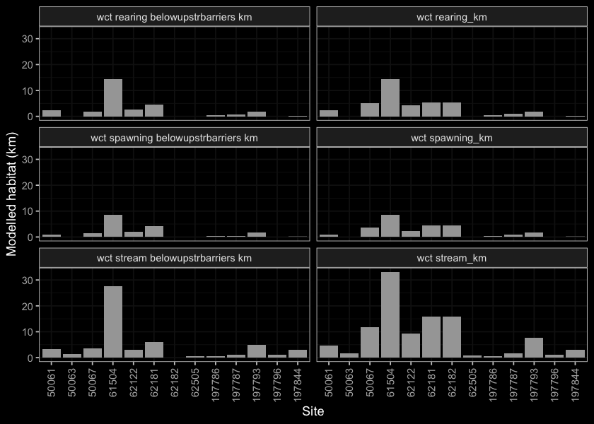
Figure 4.6: Summary of linear lengths of potential habitat upstream of habitat confirmation assessment sites estimated based on modelled discharge and gradient.