4 Results and Discussion
Results of Phase 1 and Phase 2 assessments are summarized in Figure 4.1 with additional details provided in sections below.
##make colors for the priorities
pal <-
   colorFactor(palette = c("red", "yellow", "grey", "black"),
               levels = c("high", "moderate", "low", "no fix"))

pal_phase1 <-
   colorFactor(palette = c("red", "yellow", "grey", "black"),
               levels = c("high", "moderate", "low", NA))

# tab_map_phase2 <- tab_map %>% dplyr::filter(source %like% 'phase2')
#https://stackoverflow.com/questions/61026700/bring-a-group-of-markers-to-front-in-leaflet
# marker_options <- markerOptions(
#   zIndexOffset = 1000)
tracks <- sf::read_sf("./data/habitat_confirmation_tracks.gpx", layer = "tracks")


wshd_study_areas <- sf::read_sf('data/fishpass_mapping/wshd_study_areas.geojson')
  # st_transform(crs = 4326)


map <- leaflet(height=500, width=780) %>%
  addTiles()  %>%
  # leafem::addMouseCoordinates(proj4 = 26911) %>% ##can't seem to get it to render utms yet
  # addProviderTiles(providers$"Esri.DeLorme") %>%
  addProviderTiles("Esri.WorldTopoMap", group = "Topo") %>%
  addProviderTiles("Esri.WorldImagery", group = "ESRI Aerial") %>%
  addPolygons(data = wshd_study_areas |> dplyr::filter(watershed_group_code != 'NATR'), color = "#F29A6E", weight = 1, smoothFactor = 0.5,
              opacity = 1.0, fillOpacity = 0,
              fillColor = "#F29A6E", label = wshd_study_areas$watershed_group_name) %>%
  addPolygons(data = wshds, color = "#0859C6", weight = 1, smoothFactor = 0.5,
              opacity = 1.0, fillOpacity = 0.25,
              fillColor = "#00DBFF",
              label = wshds$stream_crossing_id,
              popup = leafpop::popupTable(x = select(wshds %>% st_set_geometry(NULL),
                                                     Site = stream_crossing_id,
                                                     elev_site:area_km),
                                          feature.id = F,
                                          row.numbers = F),
              group = "Phase 2") %>%
  addLegend(
    position = "topright",
    colors = c("red", "yellow", "grey", "black"),
    labels = c("High", "Moderate", "Low", 'No fix'), opacity = 1,
    title = "Fish Passage Priorities") %>%

addCircleMarkers(data=tab_map %>%
                   dplyr::filter(source %like% 'phase1' | source %like% 'pscis_reassessments'),
                 label = tab_map %>% dplyr::filter(source %like% 'phase1' | source %like% 'pscis_reassessments') %>% pull(pscis_crossing_id),
                 # label = tab_map$pscis_crossing_id,
                 labelOptions = labelOptions(noHide = F, textOnly = TRUE),
                 popup = leafpop::popupTable(x = select((tab_map %>% st_set_geometry(NULL) %>% dplyr::filter(source %like% 'phase1' | source %like% 'pscis_reassessments')),
                                                        Site = pscis_crossing_id, Priority = priority_phase1, Stream = stream_name, Road = road_name, `Habitat value`= habitat_value, `Barrier Result` = barrier_result, `Culvert data` = data_link, `Culvert photos` = photo_link, `Model data` = model_link),
                                             feature.id = F,
                                             row.numbers = F),
                 radius = 9,
                 fillColor = ~pal_phase1(priority_phase1),
                 color= "#ffffff",
                 stroke = TRUE,
                 fillOpacity = 1.0,
                 weight = 2,
                 opacity = 1.0,
                 group = "Phase 1") %>%
  addPolylines(data=tracks,
               opacity=0.75, color = '#e216c4',
               fillOpacity = 0.75, weight=5, group = "Phase 2") %>%

addAwesomeMarkers(
    lng = as.numeric(photo_metadata$gps_longitude),
    lat = as.numeric(photo_metadata$gps_latitude),
    popup = leafpop::popupImage(photo_metadata$url, src = "remote"),
    clusterOptions = markerClusterOptions(),
    group = "Phase 2") %>%

  #commented out this section for now until tab_hab_map object is built from cost estimate table
  addCircleMarkers(
    data=tab_hab_map,
    label = tab_hab_map$pscis_crossing_id,
    labelOptions = labelOptions(noHide = T, textOnly = TRUE),
    popup = leafpop::popupTable(x = select((tab_hab_map %>% st_drop_geometry()),
                                           Site = pscis_crossing_id,
                                           Priority = priority,
                                           Stream = stream_name,
                                           Road = road_name,
                                           `Habitat (m)`= upstream_habitat_length_m,
                                           Comments = comments,
                                           `Culvert data` = data_link,
                                           `Culvert photos` = photo_link,
                                           `Model data` = model_link),
                                feature.id = F,
                                row.numbers = F),
    radius = 9,
    fillColor = ~pal(priority),
    color= "#ffffff",
    stroke = TRUE,
    fillOpacity = 1.0,
    weight = 2,
    opacity = 1.0,
    group = "Phase 2"
    ) %>%

  addLayersControl(
    baseGroups = c(
      "Esri.DeLorme",
      "ESRI Aerial"),
    overlayGroups = c("Phase 1", "Phase 2"),
    options = layersControlOptions(collapsed = F)) %>%
  leaflet.extras::addFullscreenControl() %>%
  addMiniMap(tiles = providers$"Esri.NatGeoWorldMap",
             zoomLevelOffset = -6, width = 100, height = 100)

map %>%
  hideGroup(c("Phase 2"))
Figure 4.1: Map of fish passage and habitat confirmation results
4.1 Communicate Connectivity Issues
We conducted an online presentation through FWCP to showcase the project on February 23, 2024 with over 70 people in attendance. A presentation to FWCP Peace board detailing project progress, goals and budgets was also completed on February 6, 2024.
SERNbc and McLeod Lake have been actively engaging with the following groups through numerous meetings, emails and phone calls to build awareness for the initiative, solicit input, prioritize sites, raise partnership funding and plan/implement fish passage remediations:
- McLeod Lake Indian Band members of council
- BCTS Engineering
- CN Rail
- Canadian Forest Products (Canfor)
- Sinclar Forest Projects Ltd. (Sinclar)
- Northern Engineering - Ministry of Forests
- BC Ministry of Transportation and Infrastructure
- Fish Passage Technical Working Group
- Coastal Gaslink
- British Columbia Wildlife Federation
- Planning foresters and biologists from Ministry of Forests and Ministry of Land, Water and Resource Stewardship
- Fisheries experts
- University of Northern BC
4.1.1 Collaborative GIS Environment
A summary of background information spatial layers and tables loaded to the collaborative GIS project (sern_peace_fwcp_2023) at the time of writing (2025-05-15) are included in Table 4.1.
# grab the metadata
md <- rfp::rfp_meta_bcd_xref()

# burn locally so we don't nee to wait for it
md %>%
  readr::write_csv("data/rfp_metadata.csv")
md_raw <- readr::read_csv("data/rfp_metadata.csv")
md <- dplyr::bind_rows(
md_raw,
rfp::rfp_xref_layers_custom
)
# first we will copy the doc from the Q project to this repo - the location of the Q project is outside of the repo!!
q_path_stub <- "~/Projects/gis/sern_peace_fwcp_2023/"
# this is differnet than Neexdzii Kwa as it lists layers vs tracking file (tracking file is newer than this project).
# could revert really easily to the tracking file if we wanted to.
gis_layers_ls <- sf::st_layers(paste0(q_path_stub, "background_layers.gpkg"))
gis_layers <- tibble::tibble(content = gis_layers_ls[["name"]])
# remove the `_vw` from the end of content
rfp_tracking_prep <- dplyr::left_join(
gis_layers |>
dplyr::distinct(content, .keep_all = FALSE),
md |>
dplyr::select(content = object_name, url = url_browser, description),
by = "content"
) |>
dplyr::arrange(content)
rfp_tracking_prep |>
readr::write_csv("data/rfp_tracking_prep.csv")rfp_tracking_prep <- readr::read_csv(
"data/rfp_tracking_prep.csv"
)
rfp_tracking_prep %>%
fpr::fpr_kable(caption_text = "Layers loaded to collaborative GIS project.",
footnote_text = "Metadata information for bcfishpass and bcfishobs layers can be provided here in the future but currently can usually be sourced from https://smnorris.github.io/bcfishpass/06_data_dictionary.html .",
scroll = gitbook_on)| content | url | description |
|---|---|---|
| bcfishobs.fiss_fish_obsrvtn_events_vw | https://github.com/smnorris/bcfishobs | whse_fish.fiss_fish_obsrvtn_pnt_sp points referenced to their position on the FWA stream network |
| bcfishpass.crossings_vw | https://smnorris.github.io/bcfishpass/ | Aggregated stream crossing locations. Features are aggregated from 1.PSCIS stream crossings (where possible to match to an FWA stream) 2. CABD dams (where possible to match to an FWA stream) 3. modelled road/rail/trail stream crossings 4. misc anthropogenic barriers from expert/local input |
| bcfishpass.streams_vw | https://smnorris.github.io/bcfishpass/ | View of FWA stream networks and value-added attributes. Also see https://catalogue.data.gov.bc.ca/dataset/freshwater-atlas-stream-network. |
| fwa_watershed_groups_poly | https://catalogue.data.gov.bc.ca/dataset/freshwater-atlas-watershed-groups/resource/7239c84e-418a-4a9e-97bf-61b166410384 | whse_basemapping.fwa_watershed_groups_poly. Contains polygons delimiting the watershed group boundary which is a collection of drainage area basins. In-land groups will contain a single polygon, coastal groups may contain multiple polygons (one for each island) i.e., this is a multipart polygon feature. Spatial geometry: multipart polygon |
| parameters_habitat_method | https://github.com/smnorris/bcfishpass/tree/main/parameters | List of watershed groups to process, and the IP model method to use per watershed group, where cw indicates channel width and mad indicates mean annual discharge. |
| parameters_habitat_thresholds | https://github.com/smnorris/bcfishpass/tree/main/parameters | Per-species thresholds to use for IP modelling |
| reg_legal_and_admin_boundaries.qsoi_bc_regions | https://catalogue.data.gov.bc.ca/dataset/69ea1b64-e7ce-481c-b0b5-e6450111697d | Statement of Intent Boundaries Registered with the BC Treaty Commission at date of production |
| rfp_tracking | https://github.com/NewGraphEnvironment/dff-2022/tree/master/scripts/qgis |
File tracking addition of layers to the backgroun_layers.gpkg of the project. Includes metadata related to time of creation and watershed groups used to clip layer to study area.
|
| whse_admin_boundaries.clab_indian_reserves | https://catalogue.data.gov.bc.ca/dataset/8efe9193-80d2-4fdf-a18c-d531a94196ad | Provide the administrative boundaries (extent) of Canada Lands which includes Indian Reserves. Administrative boundaries were compiled from Legal Surveys Division’s cadastral datasets and survey records archived in the Canada Lands Survey Records. See the Natural Resource Canada’s GeoGratis website, Aboriginal Lands. |
| whse_admin_boundaries.clab_national_parks | https://catalogue.data.gov.bc.ca/dataset/88e61a14-19a0-46ab-bdae-f68401d3d0fb | This dataset provides the administrative boundaries of National Parks and National Park Reserves within the province of British Columbia. Administrative boundaries were compiled from Legal Surveys Division’s cadastral datasets and survey records archived in the Canada Lands Survey Records. Canada Lands Administrative Boundaries (CLAB) were adjusted to match British Columbia’s authoritative base mapping features. The Fresh Water Atlas (FWA) was used for streams, rivers, coastlines, and height of land. The Integrated Cadastral Fabric (ICF) was used for parcel boundaries. Tantalis Cadastre was used where ICF parcels were not available. |
| whse_basemapping.bcgs_20k_grid | https://catalogue.data.gov.bc.ca/dataset/a61976ac-d8e8-4862-851e-d105227b6525 | BCGS 1:20,000 scale grid. The British Columbia Geographic System is a geographic system in which the coverage in minutes and seconds of longitude is double the coverage in minutes and seconds of latitude for sheets at all scales |
| whse_basemapping.bcgs_5k_grid | https://catalogue.data.gov.bc.ca/dataset/8376b3b3-3103-4055-a952-ca7e937e8171 | British Columbia Geographic System 1:5,000 scale mapsheet grid. Each mapsheet is one fourth of a 1:10,000 mapsheet numbered 1 through 4. The neatlines were defined and created in geographic units and reprojected to BC Albers. Each of the mapsheets is 0.75 minutes (45 seconds) latitude by 1.50 minutes (90 seconds) longitude. The British Columbia Geographic System is a geographic system in which the coverage in minutes and seconds of longitude is double the coverage in minutes and seconds of latitude for sheets at all scales |
| whse_basemapping.cwb_floodplains_bc_area_svw | https://catalogue.data.gov.bc.ca/dataset/cdf4900e-90c0-449f-beea-43b669bd76a8 | Historical floodplain boundaries in BC with a descriptive feature name for each floodplain area (i.e., 200-year floodplain, alluvial fan, or nothing/out-of-floodplain). Digitized from hardcopy 1:5,000 Floodplain Mapsheets for each project area |
| whse_basemapping.fwa_glaciers_poly | https://catalogue.data.gov.bc.ca/dataset/8f2aee65-9f4c-4f72-b54c-0937dbf3e6f7 |
Glaciers and ice masses for the province, derived from aerial imagery flown in the late 1980s and early 1990s. Please refer to the Glaciers dataset for recent glacier extents in British Columbia, and Historical Glaciers for a comparable historic view. |
| whse_basemapping.fwa_lakes_poly | https://catalogue.data.gov.bc.ca/dataset/cb1e3aba-d3fe-4de1-a2d4-b8b6650fb1f6 | All lake polygons for the province |
| whse_basemapping.fwa_manmade_waterbodies_poly | https://catalogue.data.gov.bc.ca/dataset/055fd71e-b771-4d47-a863-8a54f91a954c | All manmade waterbodies, including reservoirs and canals, for the province |
| whse_basemapping.fwa_named_streams | – | – |
| whse_basemapping.fwa_watershed_groups_poly | https://catalogue.data.gov.bc.ca/dataset/51f20b1a-ab75-42de-809d-bf415a0f9c62 | Polygons delimiting the watershed group boundary, which is a collections of drainage areas. In-land groups will contain a single polygon, coastal groups may contain multiple polygons (one for each island) |
| whse_basemapping.fwa_wetlands_poly | https://catalogue.data.gov.bc.ca/dataset/93b413d8-1840-4770-9629-641d74bd1cc6 | All wetland polygons for the province |
| whse_basemapping.gba_railway_tracks_sp | https://catalogue.data.gov.bc.ca/dataset/4ff93cda-9f58-4055-a372-98c22d04a9f8 | This layer contains railway tracks within BC from GeoBase’s National Railway Network (NRWN) dataset. |
| whse_basemapping.gba_transmission_lines_sp | https://catalogue.data.gov.bc.ca/dataset/384d551b-dee1-4df8-8148-b3fcf865096a |
High voltage electrical transmission lines for distributing power throughout the province. Lines were derived from several data sources representing unique inventories: BC Hydro, Private, Independent Power Producers, and Terrain Resource Information Management (TRIM). Voltage information is not currently available on the public version of this dataset as per publication agreement with BC Hydro. |
| whse_basemapping.transport_line | – | – |
| whse_basemapping.utmg_utm_zones_sp | https://catalogue.data.gov.bc.ca/dataset/fc999f51-306a-4adf-9b19-63b2d3c38348 | Portions of Universal Transverse Mercator Zones 7 - 12 which cover British Columbia, Northern Hemisphere only, formed into polygons, in BC Albers projection |
| whse_cadastre.pmbc_parcel_fabric_poly_svw | https://catalogue.data.gov.bc.ca/dataset/4cf233c2-f020-4f7a-9b87-1923252fbc24 |
ParcelMap BC is the current, complete and trusted mapped representation of titled and Crown land parcels across British Columbia, considered to be the point of truth for the graphical representation of property boundaries. It is not the authoritative source for the legal property boundary or related records attributes; this will always be the plan of survey or the related registry information. This particular dataset is a subset of the complete ParcelMap BC data and is comprised of the parcel fabric and attributes for over two million parcels published under the Open Government Licence - British Columbia. Notes:
|
|
whse_environmental_monitoring.ems_monitoring_locn_types_svw |
https://catalogue.data.gov.bc.ca/dataset/634ee4e0-c8f7-4971-b4de-12901b0b4be6 |
Environmental Monitoring Stations (EMS) spatial points coverage for the Province by LOCATION TYPES. The following spatial layers reference this as a data source:
|
| whse_environmental_monitoring.envcan_hydrometric_stn_sp | https://catalogue.data.gov.bc.ca/dataset/4c169515-6c41-4f6a-bd30-19a1f45cad1f | BC active and discontinued hydrometric stations (surface water level and flow data) that are part of the provincial hydrometric network managed under a national program jointly administered under a federal-provincial cost-sharing agreement with Environment and Climate Change Canada (ECCC). |
| whse_fish.fiss_obstacles_pnt_sp | https://catalogue.data.gov.bc.ca/dataset/35bbac7c-2e2f-4587-9108-f4aa1e862809 | The Provincial Obstacles to Fish Passage theme presents records of all known obstacles to fish passage from several fisheries datasets. Records from the following datasets have been included: The Fisheries Information Summary System (FISS); the Fish Habitat Inventory and Information Program (FHIIP); the Field Data Information System (FDIS) and the Resource Analysis Branch (RAB) inventory studies. The main intent of this layer is to have a single layer of all known obstacles to fish passage. It is important to note that not all waterbodies have been studied and, not all lengths of many waterbodies have been studied so there are a very high number of obstacles in the real world that are not recorded in this dataset. This layer simply reports the obstacles to fish that are known. It is also very important to note that we are acknowledging these features as obstacles to fish passage versus barriers to fish passage. This is because an obstacle may be a barrier at one time of year but not at other times depending on the volume of water present and also, what is a barrier to one species of fish is not necessarily a barrier to another species. |
| whse_fish.fiss_stream_sample_sites_sp | https://catalogue.data.gov.bc.ca/dataset/e616864b-8991-42d1-a2f9-4d4402c32be8 | This spatial layer displays stream inventory sample sites that have had full or partial surveys, and contains measurements or indicator information of the data collected at each survey site on each date. |
| whse_fish.pscis_assessment_svw | https://catalogue.data.gov.bc.ca/dataset/7ecfafa6-5e18-48cd-8d9b-eae5b5ea2881 | Points where a fish passage assessment has been performed on a stream crossing structure. These includes culverts, bridges, fords, etc. The assessments are carried out to determine whether fish are able to migrate through the structure. |
| whse_fish.pscis_design_proposal_svw | https://catalogue.data.gov.bc.ca/dataset/0c9df95f-a2da-4a7d-b9cb-fea3e8926661 | Points where a fish passage assessment has been performed on a stream crossing structure and found to be a failure. Design points have been identified as a priority for remediation based on a variety of potential criteria: quality of habitat upstream, quantity of fish habitat upstream, number and importance of species present, operational plans for the road cost of the proposed remediation, etc. They are sites where the amount of habitat to be gained by remediation has been confirmed and where a design has actually been completed. |
| whse_fish.pscis_habitat_confirmation_svw | https://catalogue.data.gov.bc.ca/dataset/572595ab-0a25-452a-a857-1b6bb9c30495 | Points where an evaluation of the fish habitat up and downstream of a road crossing have been carried out. Phase 2 of 4 in the Fish Passage Workflow, Habitat Confirmations are done at sites where the crossing structure is known to be a failure. The Habitat Confirmation is performed to ensure that the site in question is a good candidate for moving on to the Design (Phase 3) and Remediation (Phase 4) stages of the workflow. The Habitat Confirmation confirms the crossing is a barrier, places the crossing in context with respect to other roads and crossings in the watershed and also quantifies and qualifies how much habitat will be gained if the site is fixed. |
| whse_fish.pscis_remediation_svw | https://catalogue.data.gov.bc.ca/dataset/1596afbf-f427-4f26-9bca-d78bceddf485 | Points where a barrier to fish passage has been rectified or remediated. This is the third phase in the process and can only follow after 1. An assessment has been performed on a stream crossing structure and has found that structure to be a barrier to fish passage. 2. The site has been identified as a priority for remediation based on a variety of potential criteria: quality of habitat upstream, quantity of fish habitat upstream, number and importance of species present, operational plans for the road, cost of the proposed remediation, etc. 3. a design has been created for the site |
| whse_fish.wdic_waterbody_route_line_svw | https://catalogue.data.gov.bc.ca/dataset/9c3f8dd6-d715-4e3c-aa9b-cd8e26f9906d | Stream routes. Each stream channel is represented by a single line. Derived from the Stream Centreline Network Spatial layer and based on the 1:50,000 scale Canadian National Topographic Series of Maps. |
| whse_forest_tenure.ften_range_poly_carto_vw | – | – |
| whse_forest_tenure.ften_road_section_lines_svw | https://catalogue.data.gov.bc.ca/dataset/243c94a1-f275-41dc-bc37-91d8a2b26e10 | This is a spatial layer that reflects operational activities for road sections contained within a road permit. The Forest Tenures Section (FTS) is responsible for the creation and maintenance of digital Forest Atlas files for the province of British Columbia encompassing Forest and Range Act Tenures. It also supports the forest resources programs delivered by MoFR |
| whse_forest_vegetation.veg_burn_severity_sp | https://catalogue.data.gov.bc.ca/dataset/c58a54e5-76b7-4921-94a7-b5998484e697 |
This layer is the one-year-later burn severity classification for large fires (greater than 100 ha). Burn severity mapping is conducted using best available pre- and post-fire satellite multispectral imagery acquired by the MultiSpectral Instrument (MSI) aboard the Sentinel-2 satellite or the Operational Land Imager (OLI) sensor aboard the Landsat-8 and 9 satellites. The post-fire imagery is acquired during the subsequent growing season. Mapping conducted during the subsequent growing season benefits from greater post-fire image availability and is expected to be more representative of tree mortality. Every attempt is made to use cloud, smoke, shadow and snow-free imagery that was acquired prior to September 30th.
Please note, this layer is 1-year-later burn severity dataset. The same-year burn severity mapping dataset (WHSE_FOREST_VEGETATION.VEG_BURN_SEVERITY_SAME_YR_SP) is considered an interim product to this layer. 4.1.1.1 Methodology:• Select suitable pre- and post-fire imagery or create a cloud/snow/smoke-free composite from multiple images scenes • Calculate normalized burn severity ratio (NBR) for pre- and post-fire images • Calculate difference NBR (dNBR) where dNBR = pre NBR – post NBR • Apply a scaling equation (dNBR_scaled = dNBR*1000 + 275)/5) • Apply BARC thresholds (76, 110, 187) to create a 4-class image (unburned, low severity, medium severity, and high severity) • Apply region-based filters to reduce noise • Confirm burn severity analysis results through visual quality control • Produce a vector dataset and apply Euclidian distance smoothing |
| whse_human_cultural_economic.hist_hist_trails_svw | https://catalogue.data.gov.bc.ca/dataset/98c097cf-32bc-40a6-8061-bfe97a295e37 | This dataset contains spatial and tabular data on non-archaeological historic trails in B.C. Some of these trails, or sections of trail, are defined or protected under provincial legislation such as the Heritage Conservation Act. Other trails or trail segments are recorded but not legally protected. This dataset represents line feature data (e.g. trail routes). |
| whse_imagery_and_base_maps.mot_culverts_sp | https://catalogue.data.gov.bc.ca/dataset/89d44ba6-7236-48ed-afab-f25a98c846ef | A Culvert is a pipe (less than 3m in diameter) or half-round flume used to transport or drain water under or away from the road and/or right of way. Culverts that are greater than or equal to 3m in diameter are stored in the MoT Bridge Structure Road Dataset. It is a Point feature |
| whse_imagery_and_base_maps.mot_road_structure_sp | https://catalogue.data.gov.bc.ca/dataset/86732641-963e-4329-8aeb-5bbfe35d2dde | The Road Structures on the highway that are maintained by the Ministry. Highway structures include bridges, culverts (greater than or equal to 3m diameter), retaining walls (perpendicular height greater than or equal to 2m), sign bridges, tunnels/snowsheds. Information is recorded in the Bridge Management Information System (BMIS) |
| whse_land_and_natural_resource.prot_historical_fire_polys_sp | https://catalogue.data.gov.bc.ca/dataset/22c7cb44-1463-48f7-8e47-88857f207702 | Wildfire perimeters for all fire seasons before the current year. Supplied through various sources. Not to be used for legal purposes. These perimeters may be updated periodically during the year. On April 1 of each year the previous year’s fire perimeters are merged into this dataset |
| whse_land_use_planning.rmp_ogma_non_legal_current_svw | https://catalogue.data.gov.bc.ca/dataset/f063bff2-d8dd-4cc3-b3a4-00165aba58e1 |
This ‘Current’ spatial data layer is publicly accessible, contains the most current Non-Legal Old Growth Management Area (OGMA) polygons and excludes any sensitive information. This data represents spatially defined areas of old growth forest that are identified during landscape unit planning or an operational planning process. Forest licensees are not required to follow direction provided by non-legal OGMAs when preparing FSPs, and may choose to manage required old growth biodiversity targets in other ways. OGMAs, in combination with other areas where forestry development is prevented or constrained, are used to achieve biodiversity targets. Please see the Additional Information and Object Description Comments below. |
| whse_legal_admin_boundaries.abms_municipalities_sp | https://catalogue.data.gov.bc.ca/dataset/e3c3c580-996a-4668-8bc5-6aa7c7dc4932 |
Legally defined Municipal polygons were drawn from metes and bounds descriptions as written in Letters Patent for Municipalities in the province of British Columbia. In the event of a discrepancy in the data, the metes and bounds description will prevail. Although the boundaries were drawn based on the legal metes and bounds descriptions, they may differ from how regional districts and their member municipalities and electoral areas currently view and/or manage their boundaries. Where discrepancies are noted, the Ministry of Municipal Affairs (the custodian) enters into discussion with the local governments whose boundaries are affected. In order to effect a change to the boundary, Cabinet approval is required. This is done through an Order in Council (OIC). While discrepancies to administrative boundaries are being resolved, boundaries may be adjusted on an ongoing basis until the requested changes are completed. The OIC_YEAR and OIC_NUMBER fields indicate the year that the boundary was passed under OIC and its associated number. The AFFECTED_ADMIN_AREA_ABRVN identifies the administrative areas that are affected by the OIC. See all of the administrative areas currently in the Administrative Boundaries Management System (ABMS). The complimentary point dataset that defines the administrative areas is also available. Other individual legally defined administrative area datasets are available from the following records: Regional Districts Electoral Areas [Province of British Columbia](https://catalogue.data.gov.bc.c |
| whse_legal_admin_boundaries.fnt_treaty_area_sp | https://catalogue.data.gov.bc.ca/dataset/c1a5d55e-fef9-4605-8b20-c08ed4f0c870 | This layer contains the areas within which the First Nation has a role (as described in the treaty) related to economic activities, governance activities and cultural activities |
| whse_mineral_tenure.og_pipeline_area_appl_sp | https://catalogue.data.gov.bc.ca/dataset/b02092f9-b053-438b-9e86-157477d78faa | Applications for land authorizations representing the right of way for pipeline activities. This dataset contains polygon features for proposed applications collected through the BC Energy Regulator’s Application Management System (AMS). This dataset is updated nightly. |
| whse_mineral_tenure.og_pipeline_area_permit_sp | https://catalogue.data.gov.bc.ca/dataset/e1500359-d6a6-4a80-abe6-5130361cbac5 | Land authorizations representing the right of way for pipeline activities. The spatial data includes polygon data for approved and post-construction pipeline rights of way collected on or after October 30, 2006. This dataset is updated nightly. |
| whse_mineral_tenure.og_pipeline_segment_permit_sp | https://catalogue.data.gov.bc.ca/dataset/ecf567ea-4901-4f51-a5b0-35959ca96c47 | Pipeline centre-lines associated with oil and gas pipeline activity and falling within the area representing the pipeline right of way. This dataset contains line features collected on or after July 11, 2016 for approved pipeline centre-line locations. The dataset is updated nightly. |
| whse_tantalis.ta_conservancy_areas_svw | https://catalogue.data.gov.bc.ca/dataset/550b3133-2004-468f-ba1f-b95d0e281e78 | TA_CONSERVANCY_AREAS_SVW contains the spatial representation (polygon) of the conservancy areas designated under the Park Act or by the Protected Areas of British Columbia Act, whose management and development is constrained by the Park Act. The view was created to provide a simplified view of this data from the administrative boundaries information in the Tantalis operational system |
| whse_tantalis.ta_park_ecores_pa_svw | https://catalogue.data.gov.bc.ca/dataset/1130248f-f1a3-4956-8b2e-38d29d3e4af7 | This dataset contains parks and protected areas managed for important conservation values and are dedicated for the preservation of their natural environments for the inspiration, use and enjoyment of the public. Places of special ecological importance are designated as ecological reserves for scientific research and educational purposes. Source data is Tantalis. *April 18, 2018: Prior to this date this dataset had one spatial boundary per park per survey plan that intersected the boundary of that park. This resulted in multiple identical boundaries for each park that had more than one survey plan overlapping it’s boundaries. The change aggregated the park data so that there is just one boundary per park with the plan numbers concatenated into a single column where each different plan number is separated by a comma. |
| whse_water_management.wris_dams_public_svw | https://catalogue.data.gov.bc.ca/dataset/bd632217-35f9-4d01-8e57-a6dbc454f236 | Province-wide SDE spatial view displaying dam locations. The public view displays a subset of the attribute data |
| whse_wildlife_inventory.spi_whf_incident_obs_ns_sv | https://catalogue.data.gov.bc.ca/dataset/50dc6ba5-8883-4bfc-b3aa-b420b190b45b |
A “wildlife habitat feature” is defined as a feature used by one or more wildlife species to meet their life history requirements. An incidental observation is a recorded detection of a species or its sign that was not a part of a formalized survey. This can occur when a non-focal species is observed during a survey for another species, outside of the study area, or as a chance observation made at random. The validity of these sightings is widely variable depending on the level of expertise of the observer and how visible the animal(s) was. This dataset is a subset of ‘Wildlife Species Inventory Incidental Observations - Non-secured’ https://catalogue.data.gov.bc.ca/dataset/7d5a14c4-3b6e-4c15-980b-68ee68796dbe, specific to publicly available Wildlife Habitat Features that may be applicable to the Kootenay Boundary Wildlife Habitat Features Order. For a comprehensive view of wildlife habitat features for the Kootenay Boundary Region that may be applicable to the Kootenay Boundary Wildlife Habitat Features Order this dataset should be viewed in conjunction with ‘Wildlife Habitat Features - WSI Surveys – Publicly Available’ https://catalogue.data.gov.bc.ca/dataset/884c20fa-17c1-491a-b5cb-993be5dff8d3 , ‘Wildlife Habitat Features – FRPA – Publicly Available’ https://catalogue.data.gov.bc.ca/dataset/9188aeff-47b0-4932-a53a-f3e70096b781 and ‘ Wildlife Habitat Features Wildlife ‘Habitat Features - FRPA – Masked – Publicly Available’ https://catalogue.data.gov.bc.ca/dataset/11911766-cb1f-4efe-b015-97ecb8dcc1d0 For more information on the Kootenay Boundary Wildlife Habitat Features Order see here: https://www2.gov.bc.ca/gov/content/environment/natural-resource-stewardship/laws-policies-standards-guidance/legislation-regulation/forest-range-practices-act/government-actions-regulation/wildlife-habitat-features/kootenay-boundary-wildlife-habitat-features- |
| whse_wildlife_management.wcp_fish_sensitive_ws_poly | https://catalogue.data.gov.bc.ca/dataset/1a560a12-9be1-49a4-971a-dbc80875a0d7 | The dataset contains approved legal boundaries for fisheries sensitive watersheds. A FSW is a mapped area with specific management objectives intended to guide development activities which may adversely impact important fish values |
| whse_wildlife_management.wcp_wha_proposed_sp | https://catalogue.data.gov.bc.ca/dataset/c2fc0a99-075e-4fdc-b85d-a8a0d88af71c | Wildlife habitat areas (WHAs) are mapped areas that are necessary to meet the habitat requirements of an Identified Wildlife element. WHAs designate critical habitats in which activities are managed to limit their impact on the Identified Wildlife element for which the area was established. The purpose of WHAs is to conserve those habitats considered most limiting to a given Identified Wildlife element. This dataset contains proposed WHAs for the entire province except for the Omenica Region as there are none in the consultation phase at this time |
| whse_wildlife_management.wcp_wildlife_habitat_area_poly | https://catalogue.data.gov.bc.ca/dataset/b19ff409-ef71-4476-924e-b3bcf26a0127 |
The dataset contains approved legal boundaries for wildlife habitat areas and specified areas for species at risk and regionally important wildlife. Additional information including approved orders associated with WHAs is available here. |
| * Metadata information for bcfishpass and bcfishobs layers can be provided here in the future but currently can usually be sourced from https://smnorris.github.io/bcfishpass/06_data_dictionary.html . |
### Interactive Dashboard {-}

# `r if(gitbook_on){knitr::asis_output("The interactive dashboard is presented in Figure \\@ref(fig:widget-planning-caption).")}else knitr::asis_output("An interactive dashboard to facilitate planning to facilitate planning within the Parsnip River, Carp River, Crooked River and Naton River watershed groups is located within the online interactive version of the report located at https://newgraphenvironment.github.io/fish_passage_peace_2023_reporting/.")`

# we have some dams that we want to exclude in this query
dams <- c('785afb41-dfdf-423c-a291-e213d4b44f26',
          '320902cd-48fc-40e5-8c0f-191086f332aa',
          '957546a9-e6c7-46bf-947a-b17d8a818d71')
# join bcfishpass to some pscis columns for the screening table
# get our dataframe to link to a map
# xings filtered by >1km of potential rearing habitat
xf <- left_join(
  bcfishpass %>%
    fpr::fpr_sp_assign_sf_from_utm(col_easting = "utm_easting", col_northing = "utm_northing") %>%
    # st_as_sf(coords = c('utm_easting', 'utm_northing'), crs = 26910, remove = F) %>%
    dplyr::filter(is.na(pscis_status) | (pscis_status != 'HABITAT CONFIRMATION' &
                                    barrier_status != 'PASSABLE' &
                                    barrier_status != 'UNKNOWN')) %>%
    dplyr::filter(bt_rearing_km > 0.499) %>%
    dplyr::filter(crossing_type_code != 'OBS') %>%
    dplyr::filter(is.na(barriers_anthropogenic_dnstr) |
         str_detect(barriers_anthropogenic_dnstr, paste(dams, collapse = "|"))) |>
    # rename(bt_rearing_km_raw = bt_rearing_km) %>%
    # mutate(bt_rearing_km = case_when(
    #   bt_rearing_km_raw >= 1 & bt_rearing_km_raw < 2 ~ '1-2km',
    #   bt_rearing_km_raw >= 2 & bt_rearing_km_raw <= 5 ~ '2-5km',
    #   bt_rearing_km_raw >= 5 & bt_rearing_km_raw <= 10 ~ '5-10km',
    #   T ~ '>10km')
    # ) %>%
    # mutate(bt_rearing_km = factor(bt_rearing_km, levels = c('1-2km', '2-5km', '5-10km', '>10km'))) %>%
    select(id = aggregated_crossings_id,
           pscis_status,
           barrier_status,
           contains('bt_'),
           utm_easting,
           utm_northing,
           gradient_gis = gradient,
           mapsheet = dbm_mof_50k_grid,
           watershed_group_code) %>%
    # need to run rowise for our fpr function to hit each row
    mutate(map_link = paste0('https://hillcrestgeo.ca/outgoing/fishpassage/projects/parsnip/archive/2022-05-27/FishPassage_', mapsheet, '.pdf')) %>%
    mutate(map_link = paste0("<a href ='", map_link,"'target='_blank'>", map_link,"</a>")) %>%
    arrange(id) %>%
    st_transform(crs = 4326),

  pscis_assessment_svw %>%
    mutate(stream_crossing_id = as.character(stream_crossing_id)) %>%
    select(
      stream_crossing_id,
      stream_name,
      road_name,
      outlet_drop,
      channel_width = downstream_channel_width,
      habitat_value_code,
      image_view_url,
      assessment_comment) %>%
    mutate(image_view_url = paste0("<a href ='", image_view_url,"'target='_blank'>",image_view_url,"</a>")) %>%
    st_drop_geometry(),

  by = c('id' = 'stream_crossing_id')) %>%
  select(id,
         stream_name,
         habitat_value = habitat_value_code,
         mapsheet,
         map_link,
         image_view_url,
         pscis_status:bt_slopeclass15_km,
         bt_spawning_km:gradient_gis,
         # bt_spawning_km,
         # bt_rearing_km_raw:gradient_gis,
         road_name:assessment_comment,
         watershed_group_code)
  # dplyr::relocate(assessment_comment, .after = last_col())


# xf %>%
#   dplyr::filter(!is.na(pscis_status))
#
# t <- xf %>%
#   group_by(bt_rearing_km) %>%
#   summarise(n = n())
# Wrap data frame in SharedData
sd <- crosstalk::SharedData$new(xf %>% dplyr::select(-mapsheet))
# Use SharedData like a dataframe with Crosstalk-enabled widgets
map <- sd %>%
leaflet(height=500) %>% #height=500, width=780
# addTiles() %>%
addProviderTiles("Esri.WorldTopoMap", group = "Topo") %>%
addProviderTiles("Esri.WorldImagery", group = "ESRI Aerial") %>%
addCircleMarkers(
label = xf$id,
labelOptions = labelOptions(noHide = T, textOnly = TRUE),
popup = leafpop::popupTable(xf %>%
st_drop_geometry() %>%
select(id,
stream_name,
bt_rearing_km,
# bt_rearing_km = bt_rearing_km_raw,
bt_spawning_km,
mapsheet,
image_view_url,
assessment_comment,
watershed_group_code),
feature.id = F,
row.numbers = F),
radius = 9,
fillColor = "red",
color= "#ffffff",
stroke = TRUE,
fillOpacity = 1.0,
weight = 2,
opacity = 1.0
) %>%
leaflet::addPolygons(data = wshd_study_areas, color = "#F29A6E", weight = 1, smoothFactor = 0.5,
opacity = 1.0, fillOpacity = 0,
fillColor = "#F29A6E", label = wshd_study_areas$watershed_group_name) %>%
leaflet::addLayersControl(
baseGroups = c(
"Esri.DeLorme",
"ESRI Aerial"),
options = layersControlOptions(collapsed = F)) %>%
leaflet.extras::addFullscreenControl(position = "bottomright")
# tbl <- reactable::reactable(
# sd,
# selection = "multiple",
# onClick = "select",
# rowStyle = list(cursor = "pointer"),
# defaultPageSize = 5
# # minRows = 10
# )
# htmltools::browsable(
# htmltools::tagList(map, tbl)
# )
widgets <- bscols(
widths = c(2, 5, 5),
filter_checkbox("label",
"Watershed Group",
sd,
~watershed_group_code),
filter_slider(id = "label",
label = "Bull Trout Rearing (km)",
sharedData = sd,
column = ~bt_rearing_km,
round = 1,
min = 0,
max = 100),
filter_slider(id = "label",
label = "Bull Trout Spawning (km)",
sharedData = sd,
column = ~bt_spawning_km,
round = 1,
max = 45)
)
htmltools::browsable(
htmltools::tagList(
widgets,
map,
datatable(sd,
class = 'cell-border stripe',
extensions=c("Scroller","Buttons","FixedColumns"),
style="bootstrap",
# class="compact",
width="100%",
rownames = F,
options=list(
deferRender=TRUE,
scrollY=300,
scrollX = T,
scroller=TRUE,
dom = 'Bfrtip',
buttons = list(
'copy',
list(
extend = 'collection',
buttons = c('csv'),
text = 'Download csv')),
fixedColumns = list(leftColumns = 2),
initComplete = JS("function(settings, json) {","$(this.api().table().container()).css({'font-size': '11px'});","}")),
escape = F)
))my_photo = 'fig/pixel.png'
my_caption= 'Dashboard to facilitate field planning for field surveys. Note that only sites modelled with no crossings and having 0.5km or more of bull trout rearing habitat (>1.5m channel width and <7.5% gradient). Full screen available through button in bottom right of map.'
knitr::include_graphics(my_photo, dpi = NA)4.2 Fish Passage Assessments
Field assessments were conducted between August 25 2023 and September 02 2023. A total of 70 Phase 1 assessments at sites not yet inventoried into the PSCIS system included 20 crossings considered “passable”, 6 crossings considered “potential” barriers and 40 crossings considered “barriers” according to threshold values based on culvert embedment, outlet drop, slope, diameter (relative to channel size) and length (BC Ministry of Environment 2011). Additionally, although all were considered fully passable, 4 crossings assessed were fords and ranked as “unknown” according to the provincial protocol. A summary of crossings assessed, a cost estimate for remediation and a priority ranking for follow up for Phase 1 sites is presented in Table 4.2. Detailed data with photos are presented in Appendix - Phase 1 Fish Passage Assessment Data and Photos.
“Barrier” and “Potential Barrier” rankings used in this project followed BC Ministry of Environment (2011) and reflect an assessment of passability for juvenile salmon or small resident rainbow trout at any flows potentially present throughout the year (Clarkin et al. 2005; Bell 1991; Thompson 2013). As noted in Bourne et al. (2011), with a detailed review of different criteria in Kemp and O’Hanley (2010), passability of barriers can be quantified in many different ways. Fish physiology (i.e. species, length, swim speeds) can make defining passability complex but with important implications for evaluating connectivity and prioritizing remediation candidates (Bourne et al. 2011; Shaw et al. 2016; Mahlum et al. 2014; Kemp and O’Hanley 2010). Washington Department of Fish & Wildlife (2009) present criteria for assigning passability scores to culverts that have already been assessed as barriers in coarser level assessments. These passability scores provide additional information to feed into decision making processes related to the prioritization of remediation site candidates and have potential for application in British Columbia.
 tab_cost_est_phase1 %>%
  select(`PSCIS ID`:`Cost Est ( $K)`) %>%
   fpr::fpr_kable(caption_text = 'Upstream habitat estimates and cost benefit analysis for Phase 1 assessments conducted on sites not yet inventoried in PSCIS. Bull trout network model (total length stream network less than 25% gradient).',
scroll = gitbook_on)| PSCIS ID | External ID | Stream | Road | Result | Habitat value | Stream Width (m) | Priority | Fix | Cost Est ( $K) |
|---|---|---|---|---|---|---|---|---|---|
| 6539 | – | Hammett Creek | Carp Lake FSR | Barrier | High | 4.5 | high | OBS | – |
| 6541 | – | Hammett Creek | Spur | Barrier | Medium | 3.8 | mod | OBS | – |
| 6543 | – | Tributary to Hammett Creek | Davie-War FSR | Barrier | High | 4.7 | high | OBS | 450 |
| 6544 | – | Tributary to Crooked River | Carp Lake FSR | Barrier | Low | 2.7 | low | OBS | 450 |
| 6546 | – | Tributary to Weedon Creek | Davie-War FSR | Barrier | Medium | 8.0 | mod | OBS | 540 |
| 6621 | – | Tributary to Weedon Creek | Davie-War FSR | Barrier | Medium | 5.6 | mod | OBS | 450 |
| 6622 | – | Tributary to Weedon Creek | Davie-Weedon Lake FSR | Barrier | High | 2.5 | high | OBS | 450 |
| 6623 | – | Tributary to Weedon Lake | Davie-Weedon Lake FSR | Barrier | Medium | 2.6 | mod | OBS | 450 |
| 198660 | 3700002 | Copper Creek | Highway 97 | Barrier | Medium | 3.7 | mod | OBS | 10500 |
| 198662 | 3700010 | Redrocky Creek | Highway 97 | Potential | Medium | 5.2 | low | OBS | 10500 |
| 198663 | 3700015 | Tributary to Crooked River | Highway 97 | Barrier | Low | 1.1 | low | SS-CBS | 1500 |
| 198664 | 3701558 | Altezega Creek | Highway 97 | Barrier | High | 3.5 | high | OBS | 10500 |
| 198666 | 2200002 | Tributary to McLeod lake | Highway 97 | Barrier | Medium | 3.0 | mod | SS-CBS | 1500 |
| 198667 | 2200779 | Tsatchuka Creek | Highway 97 | Barrier | Medium | 4.0 | mod | OBS | 10500 |
| 198668 | 2200604 | Tributary to McLeod Lake | Highway 97 | Barrier | Medium | 1.9 | mod | SS-CBS | 1500 |
| 198669 | 2200026 | Tributary to McLeod Lake | Highway 97 | Barrier | Medium | 3.3 | mod | OBS | 12000 |
| 198672 | 2200014 | Whiskers Creek | Highway 97 | Barrier | Medium | 7.0 | mod | OBS | 12000 |
| 198673 | 3702044 | Miller Creek | Highway 97 | Potential | Low | 2.1 | low | OBS | 12000 |
| 198674 | 3701553 | Miller Creek | Summit Lake Rd | Barrier | Low | 2.4 | low | OBS | 1400 |
| 198675 | 3701554 | O’Dell Creek | Highway 97 | Barrier | Medium | 1.9 | mod | SS-CBS | 1500 |
| 198677 | 3702075 | Witters Creek | Caine Creek FSR | Barrier | Medium | 2.0 | mod | OBS | 420 |
| 198678 | 3700005 | Witters Creek | Highway 97 | Barrier | Low | 2.3 | low | OBS | 10500 |
| 198679 | 3703410 | Witters Creek | Railway | Barrier | Low | 1.9 | low | SS-CBS | – |
| 198682 | 3700007 | Tributary to Crooked River | Highway 97 | Barrier | Low | 1.7 | low | SS-CBS | 1500 |
| 198683 | 3700006 | Tributary to Crooked River | Highway 97 | Potential | Medium | 3.4 | low | OBS | 10500 |
| 198684 | 3700019 | Tributary to Kerry Lake | Highway 97 | Barrier | Medium | 5.0 | mod | OBS | 420 |
| 198686 | 3700023 | Tributary to Crooked River | Highway 97 | Potential | High | 4.0 | mod | OBS | 10875 |
| 198688 | 3701948 | Tributary to Crooked River | Highway 97 | Barrier | Low | 3.9 | low | OBS | 23250 |
| 198689 | 2200009 | Tributary to McLeod Lake | Highway 97 | Barrier | High | 4.1 | high | OBS | 10500 |
| 198690 | 2200012 | Tributary to McLeod lake | Highway 97 | Barrier | Low | 2.5 | low | SS-CBS | 1500 |
| 198691 | 3702657 | Tributary to Kerry Lake | Kerry FSR | Barrier | Low | 1.0 | low | SS-CBS | 100 |
| 198692 | 3702663 | Tributary to Kerry Lake | Kerry FSR | Barrier | Medium | 3.6 | mod | OBS | 390 |
| 198693 | 3702665 | Tributary to Kerry Lake | Kerry FSR | Barrier | Low | 3.5 | low | OBS | 420 |
| 198694 | 3703459 | Tributary to Altezega Creek | Firth Lake FSR | Barrier | High | 2.2 | high | OBS | 420 |
| 198696 | 3702446 | Tributary to Weedon Lake | Davie-Weedon Lake FSR | Barrier | Low | 0.0 | low | SS-CBS | 100 |
| 198697 | 3702959 | Tributary to Weedon Creek | Davie-Weedon Lake FSR | Barrier | Medium | 3.4 | mod | OBS | 420 |
| 198698 | 3702445 | Tributary to Weedon Lake | Davie-Weedon Lake FSR | Barrier | Medium | 3.5 | mod | OBS | 420 |
| 198699 | 3703222 | Tributary to Davie Lake | Davie Lake FSR | Barrier | Medium | 2.3 | mod | OBS | 420 |
| 198701 | 3703203 | Tributary to Davie Lake | Davie Lake FSR | Barrier | Low | 1.2 | low | SS-CBS | 100 |
| 198702 | 2200301 | Tributary to Hammett Creek | Carp Lake FSR | Barrier | Medium | 3.0 | mod | OBS | 420 |
| 198704 | 2200987 | Tributary to Hammett Creek | Davie-War FSR | Barrier | Low | 1.0 | low | SS-CBS | 100 |
| 198706 | 3702455 | Tributary to Weedon Lake | David-Weedon Lake FSR | Barrier | Medium | 10.0 | mod | OBS | 480 |
| 198708 | 3703210 | Tributary to Davie Lake | David Lake FSR | Barrier | Medium | 2.4 | mod | OBS | 420 |
| 198709 | 3703209 | Tributary to Crooked River | Davie Lake FSR | Potential | Low | 4.0 | low | OBS | 420 |
| 198711 | 3702919 | Tributary to Crooked River | Davie-Muskeg FSR | Barrier | Medium | 4.3 | mod | OBS | 390 |
| 198712 | 3702923 | Tributary to Crooked River | Davie-Muskeg FSR | Barrier | Medium | 2.7 | mod | SS-CBS | 100 |
| 198713 | 3702924 | Tributary to Crooked River | Davie-Muskeg FSR | Barrier | Medium | 3.4 | mod | SS-CBS | 100 |
| 198714 | 2023083101 | Tributary to McLeod Lake | Campground Rd | Barrier | Medium | 2.3 | mod | OBS | – |
| 198716 | 3700333 | 42 Mile Creek | Unnamed | Barrier | Low | 1.6 | low | SS-CBS | 100 |
| 198717 | 3700192 | Tributary to Crooked River | Spur | Barrier | Low | 1.2 | low | SS-CBS | 100 |
| 198719 | 3702074 | Balsam Creek | Caine Creek FSR | Barrier | Low | 1.2 | low | SS-CBS | – |
| 198720 | 3702077 | Enquist Creek | Caine Creek FSR | Potential | Medium | 1.9 | low | SS-CBS | 100 |
| 198721 | 3702073 | Tributary to Summit Lake | Caine Creek FSR | Barrier | Low | 1.7 | low | SS-CBS | 100 |
| 198723 | 3701268 | Tributary to Altezega Creek | Spur | Barrier | High | 2.2 | high | OBS | 420 |
4.3 Habitat Confirmation Assessments
During 2023 field assessments, habitat confirmation assessments were conducted at 5 sites in the Parsnip River, Carp River and Crooked River watershed groups. A total of approximately 3km of stream was assessed. Georeferenced field maps are presented in Attachment 1.
As collaborative decision making was ongoing at the time of reporting, site prioritization can be considered preliminary. In total, 0 crossings were rated as high priorities for proceeding to design for replacement, 4 crossings were rated as moderate priorities, and 1 crossings were rated as low priorities. Results are summarized in Figure 4.1 and Tables 4.3 - 4.4 with raw habitat and fish sampling data included in digital format here. A summary of preliminary modelling results illustrating quantities of bull trout spawning and rearing habitat potentially available upstream of each crossing as estimated by measured/modelled channel width and upstream accessible stream length are presented in Figure 4.2. Detailed information for each site assessed with Phase 2 assessments (including maps) are presented within site specific appendices to this document.
table_phase2_overview <- function(dat, caption_text = '', font = font_set, scroll = TRUE){
  dat2 <- dat %>%
    kable(caption = caption_text, booktabs = T, label = NA) %>%
    kableExtra::kable_styling(c("condensed"),
                              full_width = T,
                              font_size = font) %>%
    kableExtra::column_spec(column = c(9), width_min = '1.5in') %>%
    kableExtra::column_spec(column = c(5), width_max = '1in')

  if(identical(scroll,TRUE)){
    dat2 <- dat2 %>%
      kableExtra::scroll_box(width = "100%", height = "500px")
  }
  dat2
}

tab_overview %>%
  select(-Tenure) %>%
  table_phase2_overview(caption_text = 'Overview of habitat confirmation sites. Bull trout rearing model used for habitat estimates (see references for minimum width and maximum gradient used in model)',
scroll = gitbook_on)| PSCIS ID | Stream | Road | UTM (11U) | Fish Species | Habitat Gain (km) | Habitat Value | Priority | Comments |
|---|---|---|---|---|---|---|---|---|
| 198666 | Tributary to McLeod Lake | Highway 97 | 497881 6093710 | RB | 4.7 | Medium | moderate | Beaver influenced wetland area upstream for entire length. Some flowing sections for the bottom 75 m or so but no gravels or well defined deep pools present. 13:33:57 |
| 198687 | 42 Mile Creek | Highway 97 | 510950 6072479 | RB | 3.9 | High | moderate | Few patches of gravel suitable for rainbow spawning. Very little deep pools suitable for overwintering. Moderate flow with some undercut banks and functional large woody debris. Fry spotted near culvert and ~450m upstream. Stream dewaters 550m upstream of culvert. Sporadic areas with water afterwards. Healthy deciduous riparian vegetation. 09:23:38 |
| 198694 | Tributary to Altezega Creek | Firth Lake FSR | 513783 6067301 | – | 4.4 | High | moderate | Small fish spotted periodically throughout survey. A lot of blowndown first 250m, creating cover across channel and adding complexity to stream habitat. Some deep pools suitable for overwintering. A couple areas with patches of gravel for spawning. No major barriers present. Low gradient stream with riffle pool morphology, no steps or cascades. Overall, habitat rated high value. 09:47:34 |
| 198714 | Tributary to McLeod Lake | Campground Rd | 497758 6093674 | RB | – | Medium | moderate | Nice stream with abundant gravel throughout. No pool habitat. Stream potentially dredged through campground as channel is very straight and entrenched. |
| 198723 | Tributary to Altezega Creek | Spur | 513674 6067268 | – | – | High | – | – |
fpr::fpr_table_cv_summary(dat = pscis_phase2) %>%
fpr::fpr_kable(caption_text = 'Summary of Phase 2 fish passage reassessments.', scroll = F)| PSCIS ID | Embedded | Outlet Drop (m) | Diameter (m) | SWR | Slope (%) | Length (m) | Final score | Barrier Result |
|---|---|---|---|---|---|---|---|---|
| 198666 | No | 0.65 | 1.20 | 2.50 | 0.5 | 60 | 32 | Barrier |
| 198687 | Yes | 0.00 | 2.00 | 1.25 | 0.5 | 26 | 11 | Passable |
| 198694 | No | 0.00 | 0.75 | 2.93 | 2.0 | 12 | 21 | Barrier |
| 198714 | No | 0.00 | 1.20 | 1.92 | 5.0 | 8 | 26 | Barrier |
| 198723 | No | 0.00 | 1.40 | 1.57 | 1.0 | 5 | 21 | Barrier |
tab_cost_est_phase2_report %>%
  fpr::fpr_kable(caption_text = 'Cost benefit analysis for Phase 2 assessments. Bull trout rearing model used (total length of stream segments <7.5% gradient)',
scroll = FALSE)| PSCIS ID | Stream | Road | Result | Habitat value | Stream Width (m) | Fix | Cost Est (in $K) | Habitat Upstream (m) | Cost Benefit (m / $K) | Cost Benefit (m2 / $K) |
|---|---|---|---|---|---|---|---|---|---|---|
| 198666 | Tributary to McLeod Lake | Highway 97 | Barrier | Medium | 3.4 | SS-CBS | 1500 | 4680 | 3120.0 | 4680.0 |
| 198687 | 42 Mile Creek | Highway 97 | Passable | High | 3.1 | – | – | 3940 | – | – |
| 198694 | Tributary to Altezega Creek | Firth Lake FSR | Barrier | High | 2.7 | OBS | 420 | 4370 | 10404.8 | 11445.2 |
| 198714 | Tributary to McLeod Lake | Campground Rd | Barrier | Medium | 2.8 | OBS | – | – | – | – |
| 198723 | Tributary to Altezega Creek | Spur | Barrier | High | 2.4 | OBS | 420 | – | – | – |
tab_hab_summary %>%
  # dplyr::filter(Location %ilike% 'upstream') %>%
  # select(-Location) %>%
  rename(`PSCIS ID` = Site, `Length surveyed upstream (m)` = `Length Surveyed (m)`) %>%
fpr::fpr_kable(caption_text = 'Summary of Phase 2 habitat confirmation details.', scroll = FALSE)| PSCIS ID | Location | Length surveyed upstream (m) | Channel Width (m) | Wetted Width (m) | Pool Depth (m) | Gradient (%) | Total Cover | Habitat Value |
|---|---|---|---|---|---|---|---|---|
| 198666 | Upstream | 220 | 3.4 | 2.5 | – | 1.5 | moderate | medium |
| 198666 | Upstream2 | 150 | 3.2 | 2.4 | 0.7 | 4.0 | – | medium |
| 198666 | Upstream3 | 250 | 3.6 | 3.3 | 0.4 | 1.5 | moderate | medium |
| 198687 | Downstream | 200 | 2.9 | 1.6 | 0.6 | 2.2 | abundant | – |
| 198687 | Upstream | 600 | 3.1 | 1.7 | 0.3 | 2.8 | moderate | medium |
| 198694 | Upstream | 650 | 2.7 | 1.9 | 0.4 | 2.8 | abundant | medium |
| 198714 | Upstream | 250 | 2.8 | 1.9 | – | 2.7 | moderate | medium |
| 198723 | Upstream | 200 | 2.4 | 1.5 | – | 1.0 | moderate | medium |
fpr::fpr_table_wshd_sum() %>%
  fpr::fpr_kable(caption_text = paste0('Summary of watershed area statistics upstream of Phase 2 crossings.'),
footnote_text = 'Elev P60 = Elevation at which 60% of the watershed area is above', scroll = F, scroll_box_height = "300px")| Site | Area Km | Elev Site | Elev Max | Elev Median | Elev P60 | Aspect |
|---|---|---|---|---|---|---|
| 125231 | 4.0 | 754 | 1605 | 1183 | 1115 | SSE |
| 125261 | 23.5 | 730 | 1137 | 844 | 835 | SSW |
| 198666 | 11.0 | 685 | 1128 | 837 | 796 | SSW |
| 198687 | 9.8 | 692 | 1066 | 909 | 892 | SSW |
| 198694 | 6.4 | 696 | 1082 | 864 | 840 | SSW |
| 198723 | 6.4 | 696 | 1082 | 864 | 840 | SSW |
| * Elev P60 = Elevation at which 60% of the watershed area is above |
bcfp_xref_plot <- xref_bcfishpass_names %>%
  dplyr::filter(!is.na(id_join) &
           !bcfishpass %ilike% 'below' &
           !bcfishpass %ilike% 'all' &
           !bcfishpass %ilike% '_ha' &
           (bcfishpass %ilike% 'rearing' |
              bcfishpass %ilike% 'spawning'))

bcfishpass_phase2_plot_prep <- bcfishpass %>%
  mutate(across(where(is.numeric), round, 1)) %>%
    dplyr::filter(stream_crossing_id %in% (pscis_phase2 %>% pull(pscis_crossing_id))) %>%
  select(stream_crossing_id, all_of(bcfp_xref_plot$bcfishpass)) %>%
  # dplyr::filter(stream_crossing_id != 197665) %>%
  mutate(stream_crossing_id = as.factor(stream_crossing_id)) |>
  pivot_longer(cols = bt_rearing_km:bt_spawning_km)  %>%
  dplyr::filter(value > 0.0 &
           !is.na(value)
         , !name %ilike% 'sk'
         ) %>%
  mutate(
    # name = stringr::str_replace_all(name, '_belowupstrbarriers_km', ''),
         name = stringr::str_replace_all(name, '_rearing', ' rearing'),
         name = stringr::str_replace_all(name, '_spawning', ' spawning'))
    # rename('Habitat type' = name,
    #        "Habitat (km)" = value)


 bcfishpass_phase2_plot_prep %>%
  ggplot(aes(x = stream_crossing_id, y = value)) +
  geom_bar(stat = "identity")+
  facet_wrap(~name)+
  # ggdark::dark_theme_bw(base_size = 11)+
   # theme(axis.text.x=element_text(angle=90, hjust=1, vjust=0.5)) +
  labs(x = "Site", y = "Modelled habitat (km)")  +
  cowplot::theme_minimal_hgrid() +
  cowplot::panel_border()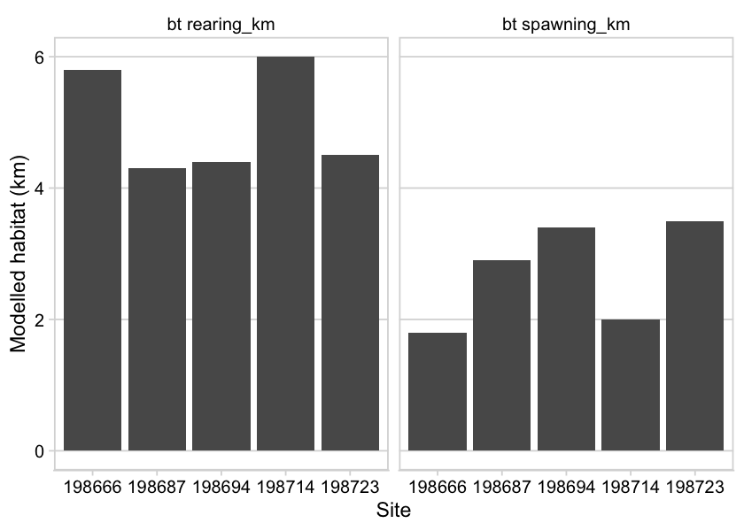
Figure 4.2: Summary of potential habitat upstream of habitat confirmation assessment sites estimated based on modelled channel width and upstream channel length.
4.4 Engineering Design
In 2024, Canfor will replace crossing 125231 (Tributary to Table River) at km21 on the Chuchinka-Table FSR with a bridge. An engineering design was completed in 2023 with some of the materials purchased for the replacement funded through this project. More detail on the site is presented in the appendix of this report titled “Tributary to the Table River - 125231 - Appendix”.
4.5 Remediations
In 2023, BCTS was able to use our project documentation to provide justification for investments in road deactivation leading to the restoration of fish passage at numerous crossings in the Parsnip River watershed including two sites ranked as priorities as part of habitat confirmation assessments documented in the FWCP funded A. Irvine (2020).
Crossing 125345, located on a tributary to the Parsnip River, was removed (along with four other culverts) during deactivation of approximately 9km of the Chuchinka-Colbourne FSR from Reynolds Creek south to approximately 9km north of the Anzac River. The site had been prioritized in A. Irvine (2020) with that report available here.
Crossing 125403, located on a tributary to the Parsnip River, was removed (along with dozens of other culverts) during deactivation of approximately 17km of the Hodda FSR. The site had been prioritized in A. Irvine (2020) with that report available here.
4.6 Monitoring
Fish sampling was conducted at a tributary to Table River (PSCIS 125231) Fern Creek (PSCIS 125261) to serve as baseline monitoring before structure replacements. Sampling was planned at a tributary to Missinka River (PSCIS 125179) however the site was inacessible due to a forest fire in the area.
Electrofishing was conducted at 12 sites with a total of 171 fish captured. Fork length data was used to delineate rainbow trout based on life stages: fry (0 to 65mm), parr (>65 to 110mm), juvenile (>110mm to 140mm) and adult (>140mm) by visually assessing the histograms presented in Figure 4.3. A summary of sites assessed are included in Table 4.8 and raw data is provided in Attachment 3. A summary of density results for all life stages combined of select species is also presented in Figure 4.4.
Detailed results for tributary to Table River (PSCIS 125231) are presented in the appendix to this report titled “Tributary to the Table River - 125231 - Appendix”. Results for Fern Creek (PSCIS 125261) are presented in “Fern Creek - 125261 - Appendix”.
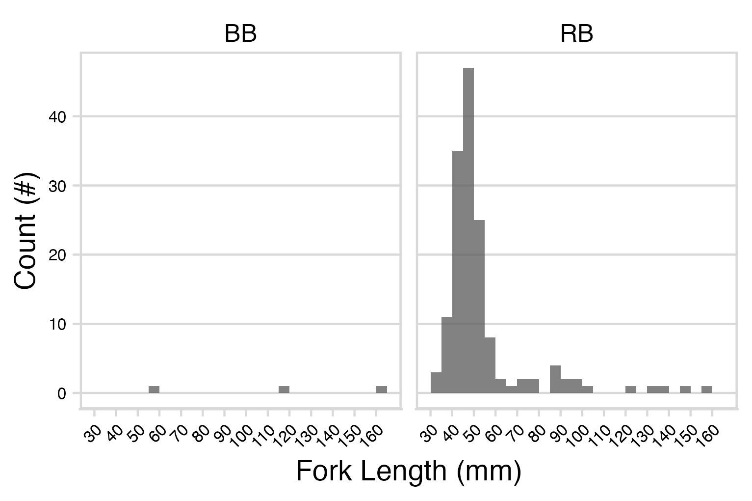
Figure 4.3: Histograms of fish lengths by species. Fish captured by electrofishing during habitat confirmation assessments.
| site | passes | ef_length_m | ef_width_m | area_m2 | enclosure |
|---|---|---|---|---|---|
| 125231_ds_ef1 | 1 | 10 | 1.6 | 16.0 | open |
| 125231_ds_ef2 | 1 | 12 | 2.6 | 31.2 | open |
| 125231_ds_ef3 | 1 | 17 | 2.2 | 37.4 | open |
| 125231_us_ef1 | 1 | 15 | 1.9 | 28.5 | open |
| 125231_us_ef2 | 1 | 19 | 1.9 | 36.1 | open |
| 125231_us_ef3 | 1 | 29 | 1.7 | 49.3 | open |
| 125261_ds_ef1 | 1 | 21 | 4.3 | 90.3 | open |
| 125261_ds_ef2 | 1 | 35 | 3.5 | 122.5 | open |
| 125261_ds_ef3 | 1 | 14 | 2.8 | 39.2 | open |
| 125261_us_ef1 | 1 | 13 | 3.8 | 49.4 | open |
| 125261_us_ef2 | 1 | 18 | 2.4 | 43.2 | open |
| 125261_us_ef3 | 1 | 16 | 4.3 | 68.8 | open |
plot_fish_box_all <-  fish_abund %>% #tab_fish_density_prep
  dplyr::filter(
    !species_code %in% c('MW', 'SU', 'NFC', 'CT', 'LSU')
  ) %>%
  ggplot(., aes(x = location, y =density_100m2)) +
  geom_boxplot()+
  facet_grid(site ~ species_code, scales ="fixed", #life_stage
             as.table = T)+
  # theme_bw()+
  # theme(legend.position = "none", axis.title.x=element_blank()) +
  # geom_dotplot(binaxis='y', stackdir='center', dotsize=1)+
  ylab(expression(Density ~ (Fish/100 ~  m^2))) +
  # ggdark::dark_theme_bw()
  cowplot::theme_minimal_hgrid() +
  cowplot::panel_border()

plot_fish_box_all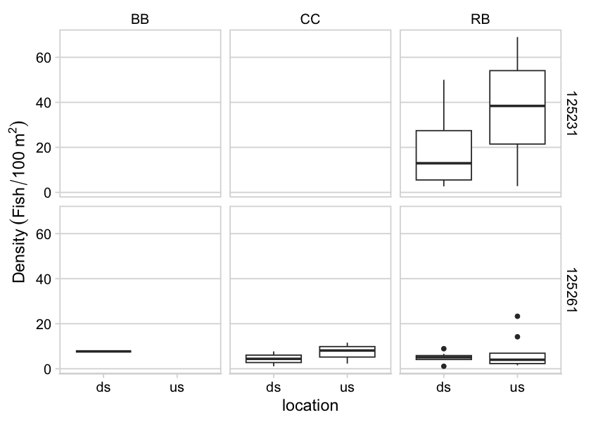
Figure 4.4: Boxplots of densities (fish/100m2) of fish captured by electrofishing during habitat confirmation assessments.
4.7 Climate Change Risk Assessment
Preliminary climate change risk assessment data is presented below. Phase 1 sites are presented in Table 4.9, and Phase 2 sites are in Table 4.10. Data can be considered preliminary and a starting point for quantification of risk factors through future adaptive management.
tab_moti_phase1 %>%
  select(-contains('Describe'), -contains('Crew')) %>%
  rename(Site = pscis_crossing_id,
         'External ID' = my_crossing_reference,
         `MoTi ID` = moti_chris_culvert_id,
         Stream = stream_name,
         Road = road_name) %>%
  mutate(across(everything(), as.character)) %>%
  tibble::rownames_to_column() %>%
  df_transpose() %>%
  janitor::row_to_names(row_number = 1) %>%
  fpr::fpr_kable(scroll = gitbook_on,
caption_text = 'Preliminary climate change risk assessment data for Ministry of Transportation and Infrastructure sites (Phase 1 PSCIS)')| Site | 198666 | 198689 | 198672 | 198669 | 198668 | 198667 | 198660 | 198680 | 198678 | 198683 | 198682 | 198662 | 198663 | 198686 | 198687 | 198661 | 198717 | 198716 | 198723 | 198674 | 198675 | 198664 | 198688 | 198673 | 198719 | 198677 | 198720 | 198698 | 198711 | 198712 | 198713 | 198697 | 198709 | 198699 | 198679 | 198694 |
|---|---|---|---|---|---|---|---|---|---|---|---|---|---|---|---|---|---|---|---|---|---|---|---|---|---|---|---|---|---|---|---|---|---|---|---|---|
| External ID | 2200002 | 2200009 | 2200014 | 2200026 | 2200604 | 2200779 | 3700002 | 3700003 | 3700005 | 3700006 | 3700007 | 3700010 | 3700015 | 3700023 | 3700024 | 3700034 | 3700192 | 3700333 | 3701268 | 3701553 | 3701554 | 3701558 | 3701948 | 3702044 | 3702074 | 3702075 | 3702077 | 3702445 | 3702919 | 3702923 | 3702924 | 3702959 | 3703209 | 3703222 | 3703410 | 3703459 |
| MoTi ID | 1997114 | 1997018 | 1997172 | 1996861 | 1996852 | 1997066 | 1997081 | 1997273 | 1997258 | 1997146 | 1997232 | 3759 | 1996752 | 1997085 | 1997302 | 1997003 | – | – | – | 3440699 | 1996948 | 2434 | 1997288 | 1996888 | – | – | – | – | – | – | – | – | – | – | – | – |
| Stream | Tributary to McLeod lake | Tributary to McLeod Lake | Whiskers Creek | Tributary to McLeod Lake | Tributary to McLeod Lake | Tsatchuka Creek | Copper Creek | Neilson Creek | Witters Creek | Tributary to Crooked River | Tributary to Crooked River | Redrocky Creek | Tributary to Crooked River | Tributary to Crooked River | 42 Mile Creek | Tributary to Crooked River | Tributary to Crooked River | 42 Mile Creek | Tributary to Altezega Creek | Miller Creek | O’Dell Creek | Altezega Creek | Tributary to Crooked River | Miller Creek | Balsam Creek | Witters Creek | Enquist Creek | Tributary to Weedon Lake | Tributary to Crooked River | Tributary to Crooked River | Tributary to Crooked River | Tributary to Weedon Creek | Tributary to Crooked River | Tributary to Davie Lake | Witters Creek | Tributary to Altezega Creek |
| Road | Highway 97 | Highway 97 | Highway 97 | Highway 97 | Highway 97 | Highway 97 | Highway 97 | Highway 97 | Highway 97 | Highway 97 | Highway 97 | Highway 97 | Highway 97 | Highway 97 | Highway 97 | Highway 97 | Spur | Unnamed | Spur | Summit Lake Rd | Highway 97 | Highway 97 | Highway 97 | Highway 97 | Caine Creek FSR | Caine Creek FSR | Caine Creek FSR | Davie-Weedon Lake FSR | Davie-Muskeg FSR | Davie-Muskeg FSR | Davie-Muskeg FSR | Davie-Weedon Lake FSR | Davie Lake FSR | Davie Lake FSR | Railway | Firth Lake FSR |
| Erosion (scale 1 low - 5 high) | 1 | 1 | 1 | 1 | 1 | 1 | 1 | 1 | 2 | 1 | 2 | 1 | 1 | 3 | 1 | 1 | 1 | 1 | 2 | 2 | 2 | 1 | 1 | 1 | 2 | 1 | 1 | 1 | 5 | 2 | 2 | 1 | 3 | 1 | 1 | 2 |
| Embankment fill issues 1 (low) 2 (medium) 3 (high) | 1 | 3 | 1 | 1 | 1 | 1 | 1 | 1 | 2 | 1 | 2 | 2 | 1 | 3 | 1 | 1 | 3 | 1 | 1 | 2 | 1 | 1 | 1 | 1 | 1 | 1 | 1 | 1 | 2 | 2 | 1 | 1 | 2 | 1 | 1 | 2 |
| Blockage Issues 1 (0-30%) 2 (>30-75%) 3 (>75%) | 1 | 1 | 2 | 2 | 1 | 3 | 1 | 1 | 1 | 1 | 2 | 1 | 1 | 3 | 1 | 2 | 1 | 1 | 1 | 1 | 1 | 1 | 2 | 2 | 2 | 2 | 1 | 2 | 2 | 3 | 1 | 1 | 1 | 1 | 1 | 1 |
| Condition Rank = embankment + blockage + erosion | 3 | 5 | 4 | 4 | 3 | 5 | 3 | 3 | 5 | 3 | 6 | 4 | 3 | 9 | 3 | 4 | 5 | 3 | 4 | 5 | 4 | 3 | 4 | 4 | 5 | 4 | 3 | 4 | 9 | 7 | 4 | 3 | 6 | 3 | 3 | 5 |
| Likelihood Flood Event Affecting Culvert (scale 1 low - 5 high) | 1 | 5 | 1 | 4 | 1 | 4 | 2 | 2 | 1 | 1 | 2 | 2 | 1 | 2 | 2 | 1 | 4 | 1 | 4 | 2 | 1 | 1 | 2 | 2 | 3 | 4 | 1 | 1 | 2 | 5 | 2 | 4 | 4 | 2 | 1 | 2 |
| Consequence Flood Event Affecting Culvert (scale 1 low - 5 high) | 1 | 5 | 2 | 3 | 1 | 5 | 5 | 1 | 2 | 3 | 2 | 2 | 1 | 2 | 3 | 2 | 3 | 1 | 3 | 1 | 2 | 2 | 2 | 1 | 4 | 2 | 2 | 1 | 2 | 3 | 2 | 3 | 3 | 2 | 2 | 2 |
| Climate Change Flood Risk (likelihood x consequence) 1-6 (low) 6-12 (medium) 10-25 (high) | 1 | 25 | 2 | 12 | 1 | 20 | 10 | 2 | 2 | 3 | 4 | 4 | 1 | 4 | 6 | 2 | 12 | 1 | 12 | 2 | 2 | 2 | 4 | 2 | 12 | 8 | 2 | 1 | 4 | 15 | 4 | 12 | 12 | 4 | 2 | 4 |
| Vulnerability Rank = Condition Rank + Climate Rank | 4 | 30 | 6 | 16 | 4 | 25 | 13 | 5 | 7 | 6 | 10 | 8 | 4 | 13 | 9 | 6 | 17 | 4 | 16 | 7 | 6 | 5 | 8 | 6 | 17 | 12 | 5 | 5 | 13 | 22 | 8 | 15 | 18 | 7 | 5 | 9 |
| Traffic Volume 1 (low) 5 (medium) 10 (high) | 10 | 10 | 10 | 10 | 10 | 10 | 10 | 9 | 9 | 8 | 9 | 9 | 9 | 10 | 10 | 9 | 2 | 1 | 1 | 3 | 8 | 9 | 10 | 8 | 2 | 2 | 2 | 1 | 7 | 7 | 6 | 1 | 4 | 2 | 2 | 3 |
| Community Access - Scale - 1 (high - multiple road access) 5 (medium - some road access) 10 (low - one road access) | 10 | 5 | 5 | 5 | 5 | 5 | 9 | 10 | 9 | 10 | 7 | 10 | 10 | 5 | 5 | 10 | 10 | 9 | 8 | 7 | 9 | 7 | 5 | 8 | 10 | 8 | 10 | 9 | 1 | 2 | 1 | 9 | 8 | 5 | 9 | 8 |
| Cost (scale: 1 high - 10 low) | 1 | 2 | 7 | 7 | 7 | 1 | 6 | 2 | 3 | 3 | 3 | 3 | 3 | 8 | 7 | 2 | 7 | 8 | 8 | 7 | 4 | 3 | 6 | 2 | 8 | 7 | 8 | 7 | 6 | 6 | 4 | 8 | 7 | 8 | 3 | 7 |
| Constructibility (scale: 1 difficult -10 easy) | 1 | 2 | 9 | 5 | 7 | 1 | 6 | 4 | 2 | 6 | 3 | 3 | 2 | 2 | 4 | 3 | 4 | 9 | 9 | 6 | 3 | 2 | 6 | 3 | 8 | 7 | 7 | 8 | 6 | 3 | 2 | 9 | 8 | 7 | 4 | 6 |
| Fish Bearing 10 (Yes) 0 (No) - see maps for fish points | 10 | 10 | 10 | 10 | 10 | 10 | 0 | 0 | 0 | 10 | 10 | 10 | 0 | 10 | 10 | 0 | 10 | 10 | 10 | 0 | 10 | 10 | 10 | 0 | 10 | 10 | 10 | 0 | 10 | 10 | 10 | 0 | 0 | 0 | 0 | 10 |
| Environmental Impacts (scale: 1 high -10 low) | 10 | 3 | 7 | 7 | 10 | 10 | 4 | 3 | 4 | 4 | 4 | 4 | 3 | 9 | 5 | 2 | 7 | 7 | 8 | 7 | 3 | 2 | 6 | 4 | 7 | 5 | 7 | 8 | 8 | 4 | 7 | 8 | 4 | 9 | 4 | 7 |
| Priority Rank = traffic volume + community access + cost + constructability + fish bearing + environmental impacts | 42 | 32 | 48 | 44 | 49 | 37 | 35 | 28 | 27 | 41 | 36 | 39 | 27 | 44 | 41 | 26 | 40 | 44 | 44 | 30 | 37 | 33 | 43 | 25 | 45 | 39 | 44 | 33 | 38 | 32 | 30 | 35 | 31 | 31 | 22 | 41 |
| Overall Rank = Vulnerability Rank + Priority Rank | 46 | 62 | 54 | 60 | 53 | 62 | 48 | 33 | 34 | 47 | 46 | 47 | 31 | 57 | 50 | 32 | 57 | 48 | 60 | 37 | 43 | 38 | 51 | 31 | 62 | 51 | 49 | 38 | 51 | 54 | 38 | 50 | 49 | 38 | 27 | 50 |
tab_moti_phase2 %>%
  purrr::set_names(nm = xref_moti_climate_names %>% pull(report)) %>%
  select(-my_crossing_reference) %>%
  select(-contains('Describe'), -contains('Crew')) %>%
  rename(Site = pscis_crossing_id,
         `MoTi ID` = moti_chris_culvert_id,
         Stream = stream_name,
         Road = road_name) %>%
  mutate(across(everything(), as.character)) %>%
  tibble::rownames_to_column() %>%
  df_transpose() %>%
  janitor::row_to_names(row_number = 1) %>%
  fpr::fpr_kable(scroll = gitbook_on,
caption_text = 'Preliminary climate change risk assessment data for habitat confirmation sites.')| Site | 198666 | 198687 | 198723 | 198694 |
|---|---|---|---|---|
| MoTi ID | 1997114 | 1997302 | – | – |
| Stream | Tributary to McLeod lake | 42 Mile Creek | Tributary to Altezega Creek | Tributary to Altezega Creek |
| Road | Highway 97 | Highway 97 | Spur | Firth Lake FSR |
| Erosion (scale 1 low - 5 high) | 1 | 1 | 2 | 2 |
| Embankment fill issues 1 (low) 2 (medium) 3 (high) | 1 | 1 | 1 | 2 |
| Blockage Issues 1 (0-30%) 2 (>30-75%) 3 (>75%) | 1 | 1 | 1 | 1 |
| Condition Rank = embankment + blockage + erosion | 3 | 3 | 4 | 5 |
| Likelihood Flood Event Affecting Culvert (scale 1 low - 5 high) | 1 | 2 | 4 | 2 |
| Consequence Flood Event Affecting Culvert (scale 1 low - 5 high) | 1 | 3 | 3 | 2 |
| Climate Change Flood Risk (likelihood x consequence) 1-6 (low) 6-12 (medium) 10-25 (high) | 1 | 6 | 12 | 4 |
| Vulnerability Rank = Condition Rank + Climate Rank | 4 | 9 | 16 | 9 |
| Traffic Volume 1 (low) 5 (medium) 10 (high) | 10 | 10 | 1 | 3 |
| Community Access - Scale - 1 (high - multiple road access) 5 (medium - some road access) 10 (low - one road access) | 10 | 5 | 8 | 8 |
| Cost (scale: 1 high - 10 low) | 1 | 7 | 8 | 7 |
| Constructibility (scale: 1 difficult -10 easy) | 1 | 4 | 9 | 6 |
| Fish Bearing 10 (Yes) 0 (No) - see maps for fish points | 10 | 10 | 10 | 10 |
| Environmental Impacts (scale: 1 high -10 low) | 10 | 5 | 8 | 7 |
| Priority Rank = traffic volume + community access + cost + constructability + fish bearing + environmental impacts | 42 | 41 | 44 | 41 |
| Overall Rank = Vulnerability Rank + Priority Rank | 46 | 50 | 60 | 50 |
4.8 Challenges and Opportunities
4.8.1 Costs, Timing and Partnerships
Inflation has led to significant cost increases for culvert removals and bridge installations. The projected costs for replacing culverts with bridges on small streams, on unpaved resource roads, have surged from around $180,000 in 2020 to over $400,000 in 2023. These estimates are just a fraction of the costs associated with structure replacements on railways, highways, and paved roads, which can range from near a million to tens of millions of dollars per crossing. This challenge poses a significant obstacle without straightforward mitigation. We are actively seeking new funding partners and are requesting current funders consider increasing financial support for necessary actions.
Infrastructure replacements and removals, even with full funding secured, are complex, taking several years to plan and implement, often involving multiple partners with divergent perspectives. Cost estimates stay uncertain even post-design, and numerous factors can cause delays or derail plans completely. When financial support depends on annual renewals with expectations for swift outcomes, planning becomes exceptionally challenging.
Some landowners and tenure holders lack support to implement remedial actions on the infrastructure they manage, hindering progress in fish passage restoration efforts. CN Rail infrastructure, in particular, significantly contributes to fish passage issues in the FWCP Peace Region. However, representatives from the company have communicated that historically they have been supported to complete one small fish passage remediation project per year across all of western Canada. We are exploring strategies to encourage collaborative cooperation and investment from these stakeholders.
Economic uncertainty in the forestry sector, resulting from deferred cutting permits on land tracks designated as “old-growth management areas,” has significantly impacted our study area. The British Columbia government has urged licensees to postpone harvesting in these areas until a “new approach for old growth forest management” is developed and many cutting permits have been on extended hold. Despite initial plans for the remediation of site 125000 near Arctic Lake in the summer of 2023, our project partner and forest licensee in the area, Sinclar Group, communicated in the spring of 2023 that road updates were no longer practical due to the deferrals affecting logging plans beyond the culvert. Consequently, they would not be able to allocate FWCP dollars earmarked for the site from the 2021/2022 or 2022/2023 fiscal funding pots towards the project. Fortunately, we were able to reallocate their funding to Canfor to catalyze restoration on the Missinka-Table FSR watershed instead.
4.8.2 Project Complexity and Communication
It is challenging to communicate the complexity of fish passage issues to diverse partners/stakeholders. Connectivity is on a spectrum and is not often 100% or 0% with costs of remediation high. Often there are multiple crossings on the same stream with different landowners and tenure holders for each. We will continue to build relationships and tools to help understand and communicate the issues and find ways forward that involve meaningful actions.
Collecting and presenting fish passage data poses challenges for field teams due to the large size of study areas, arduous field conditions and the complexity of stream crossing and habitat data. To address this, we are developing open-source collaborative GIS projects, mobile data collection, and iterative reporting systems to facilitate collaboration and share knowledge and methodologies with diverse partners.
4.8.3 Complimentary Programs
4.8.3.1 Arctic Grayling Research
Ongoing work in the Parsnip Core area regarding Arctic grayling abundance estimates, critical habitat and spatial ecology is providing valuable information to inform fish passage restoration efforts. Consultants and researchers have been developing multiple programs in the area with the support of the FWCP Peace Region. We are working together with these teams to incorporate their findings into our fish passage restoration planning.
4.8.3.2 BCHydro Fish Passage Program
The BC Hydro Fish Passage Program is currently working with First Nations, regulators and stakeholders in the region to develop strategies to offset impacts of fish entertainment related to the Peace Canyon and WAC Bennett dams. We met with West Moberly-DWB Limited Partnership to discuss how our programs can collaborate to identify potential sites for remediation.
4.8.3.3 Climate Change
Climate change is a significant threat to fish and fish habitat. We are working with the Ministry of Transportation and Infrastructure to incorporate climate change risk assessments into our fish passage restoration planning and plan to continue the evolution of this program into the future. Additionally, we will utilize climate modelling data to support prioritization of crossings (e.g., to support access to cold, drought resistant areas). Progress on this work is underway with details of some of the work here, here and here.