2 Background
The study area includes the Bulkley River, Zymoetz River, Kispiox River, Morice River and Kitsumkalum River watershed groups (Figure 2.1) and is within the traditional territories of the Wet’suwet’en, Gitxsan and Tsimshian.
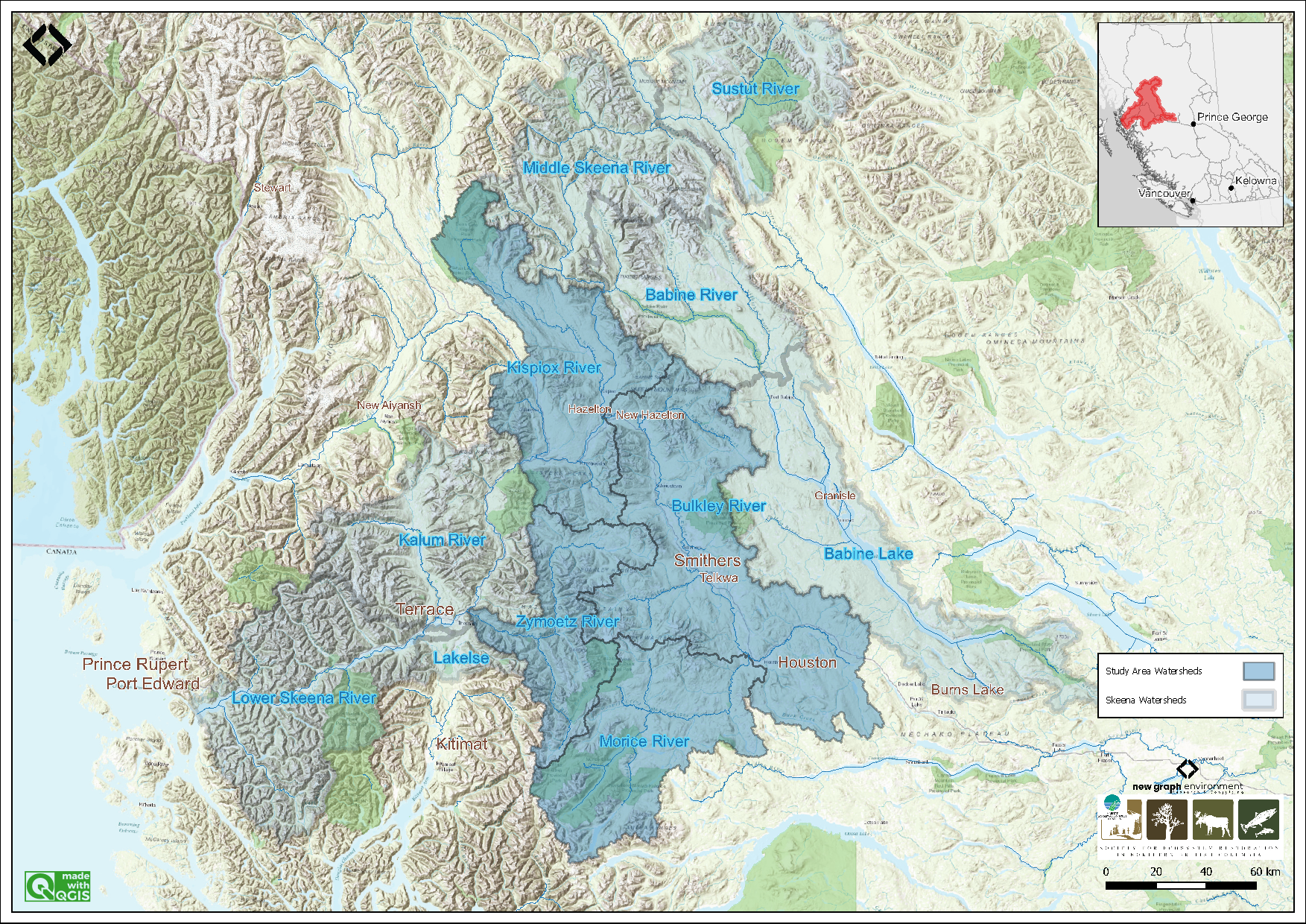
Figure 2.1: Overview map of Study Areas
2.1 Wet’suwet’en
Wet’suwet’en hereditary territory covers an area of 22,000km2 including the Bulkley River and Morice River watersheds and portions of the Nechako River watershed. The Wet’suwet’en people are a matrilineal society organized into the Gilseyhu (Big Frog), Laksilyu (Small Frog), Tsayu (Beaver clan), Gitdumden (Wolf/Bear) and Laksamshu (Fireweed) clans. Within each of the clans there are are a number of kin-based groups known as Yikhs or House groups. The Yikh is a partnership between the people and the territory. Thirteen Yikhs with Hereditary Chiefs manage a total of 38 distinct territories upon which they have jurisdiction. Within a clan, the head Chief is entrusted with the stewardship of the House territory to ensure the Land is managed in a sustainable manner. Inuk Nu’at’en (Wet’suwet’en law) governing the harvesting of fish within their lands are based on values founded on thousands of years of social, subsistence and environmental dynamics. The Yintahk (Land) is the centre of life as well as culture and it’s management is intended to provide security for sustaining salmon, wildlife, and natural foods to ensure the health and well-being of the Wet’suwet’en (Office of the Wet’suwet’en 2013; “Office of the Wet’suwet’en” 2021; FLNRORD 2017).
2.2 Gitxsan
Gitxsan means “People of the River Mist”. The Gitxsan Laxyip (traditional territories) covers an area of 33,000km2 within the Skeena River and Nass River watersheds. The Laxyip is governed by 60 Simgiigyet (Hereditary Chiefs), within the traditional hereditary system made up of Wilps (House groups). Anaat are fisheries tenures found throughout the Laxyip. Traditional governance within a matrilineal society operates under the principles of Ayookw (Gitxsan law) (“Gitxsan Huwilp Government” n.d.). Many band members live in Hazelton, Kispiox and Glen Vowell (the Eastern Gitxsan) as well as within Kitwanga, Kitwankool and Kitsegukla (the Western Gitxsan) (Powell, Jensen, and Pedersen 2018).
# Salmon is considered the source of life and always treated with high regard.  It was brought by the Raven who also taught people how to fish and hunt.

 # The original Gitxsan economy depended heavily on the trade of fish and other natural resources with neighbouring First Nations along "grease trails," which are routes named so because they carried the refined oil of the oolichan, a fish that resembles a smelt that is common in some areas of British Columbia. They are also known for their range of traditional arts
2.3 Tsimshian
The Kitsumkalum community, part of the Tsimshian Nation, maintains a rich cultural heritage rooted in ancient traditions and values. Their society, governed by Tsimshian Law (ayaawx), emphasizes strong connections through marriages, adoptions, and resource sharing with other Tsimshian tribes. The community upholds its cultural and spiritual practices, including fishing, harvesting, and land stewardship, despite the impacts of colonization (Kitsumkalum Band n.d.).
Kitsumkalum’s social structure is based on matrilineal kinship, with significant emphasis on family ties through the mother’s lineage. Their cultural identity is expressed through crest groups (pteex), lineage houses (waap), and the importance of landed property (laxyuup), which ties them to their ancestral territories. The community combines traditional governance with modern administrative functions, reflecting their resilience and commitment to preserving their heritage (Kitsumkalum Band n.d.).
The Kitsumkalum River salmon populations have been an important part of their culture and economy (A. Gottesfeld and Rabnett 2007).
2.4 Bulkley River
The Bukley River is an 8th order stream that drains an area of 7,762km2 in a generally northerly direction from Bulkley Lake on the Nechako Plateau to its confluence with the Skeena River at Hazleton. It has a mean annual discharge of 139.1 m3/s at station 08EE004 located near Quick (~27km south of Telkwa) and 19 m3/s at station 08EE003 located upstream near Houston. Flow patterns at Quick are heavily influenced by inflows from the Morice River (enters just downstream of Houston) resulting in flow patterns typical of high elevation watersheds which receive large amounts of precipitation as snow leading to peak levels of discharge during snowmelt, typically from May to July (Figures 2.2 - 2.3). The hydrograph peaks faster and generally earlier (May - June) for the Bulkley River upstream of Houston where the topography is of lower lower elevation (Figures 2.2 and 2.4).
Changes to the climate systems are causing impacts to natural and human systems on all continents with alterations to hydrological systems caused by changing precipitation or melting snow and ice increasing the frequency and magnitude of extreme events such as floods and droughts (Calvin et al. 2023; ECCC 2016). These changes are resulting in modifications to the quantity and quality of water resources throughout British Columbia and are likely to compound issues related to drought and flooding in the Bulkley River watershed where numerous water licenses are held with a potential over-allocation of flows identified during low flow periods (ILMB 2007).
The valley bottom has seen extensive settlement over the past hundred years with major population centers including the Village of Hazelton, the Town of Smithers, the Village of Telkwa and the District Municipality of Houston. As a major access corridor to northwestern British Columbia, Highway 16 and the Canadian National Railway are major linear developments that run along the Bulkley River within and adjacent to the floodplain with numerous crossing structures impeding fish access into and potentially out from important fish habitats. Additionally, as the valley bottom contains some of the most productive land in the area, there has been extensive conversion of riparian ecosystems to hayfields and pastures leading to alterations in flow regimes, increases in water temperatures, reduced streambank stability, loss of overstream cover and channelization (ILMB 2007; Wilson and Rabnett 2007).
knitr::include_graphics("fig/hydrograph_08EE004.png")
knitr::include_graphics("fig/pixel.png")
knitr::include_graphics("fig/hydrograph_08EE003.png")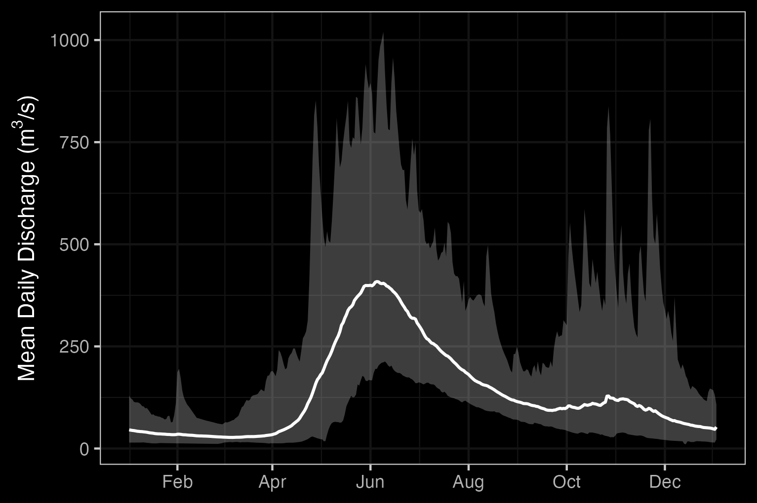
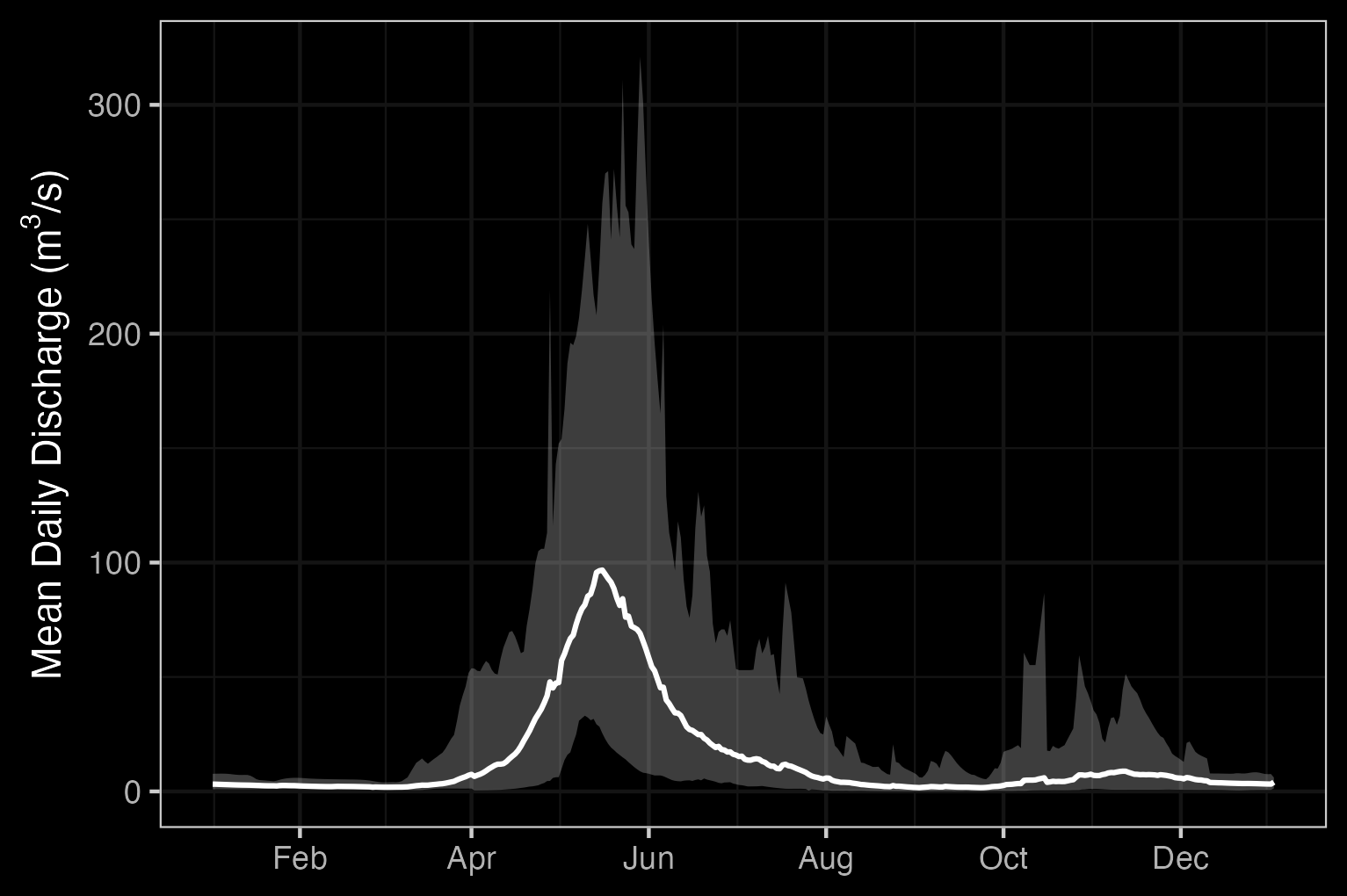
Figure 2.2: Hydrograph for Bulkley River at Quick (Station #08EE004) and near Houston (Station #08EE003).
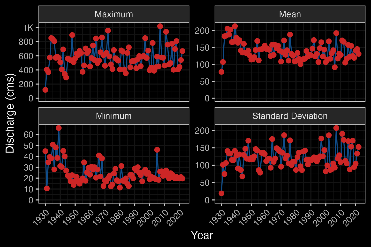
Figure 2.3: Bulkley River At Quick (Station #08EE004 - Lat 54.61861 Lon -126.89997). Available daily discharge data from 1930 to 2022.
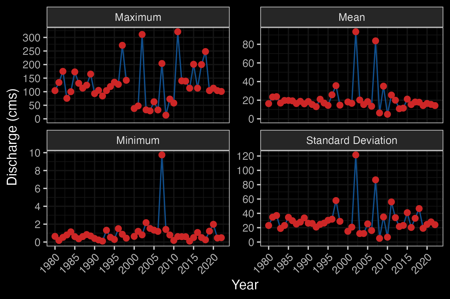
Figure 2.4: Bulkley River Near Houston (Station #08EE003 - Lat 54.39938 Lon -126.71941). Available daily discharge data from 1980 to 2022.
2.5 Morice River
The Morice River watershed drains 4,379km2 of Coast Mountains and Interior Plateau in a generally south-eastern direction. The Morice River is an 8th order stream that flows approximatley 80km from Morice Lake to the confluence with the upper Bulkley River just north of Houston. Major tributaries include the Nanika River, the Atna River, Gosnell Creek and the Thautil River. There area numerous large lakes situated on the south side of the watershed including Morice Lake, McBride Lake, Stepp Lake, Nanika Lake, Kid Price Lake, Owen Lake and others. There is one active hydrometric station on the mainstem of the Morice River near the outlet of Morice Lake and one historic station that was located at the mouth of the river near Houston that gathered data in 1971 only (Canada 2024). An estimate of mean annual discharge for the one year of data available for the Morice near it’s confluence with the Bulkley River is 113 m3/s. Mean annual discharge is estimated at 75 m3/s at station 08ED002 located near the outlet of Morice Lake. Flow patterns are typical of high elevation watersheds influenced by coastal weather patterns which receive large amounts of winter precipitation as snow in the winter and large precipitation events in the fall. This leads to peak levels of discharge during snowmelt, typically from May to July with isolated high flows related to rain and rain on snow events common in the fall (Figures 2.5 - 2.6).
knitr::include_graphics("fig/hydrograph_08ED003.png")
knitr::include_graphics("fig/pixel.png")
knitr::include_graphics("fig/hydrograph_08ED002.png")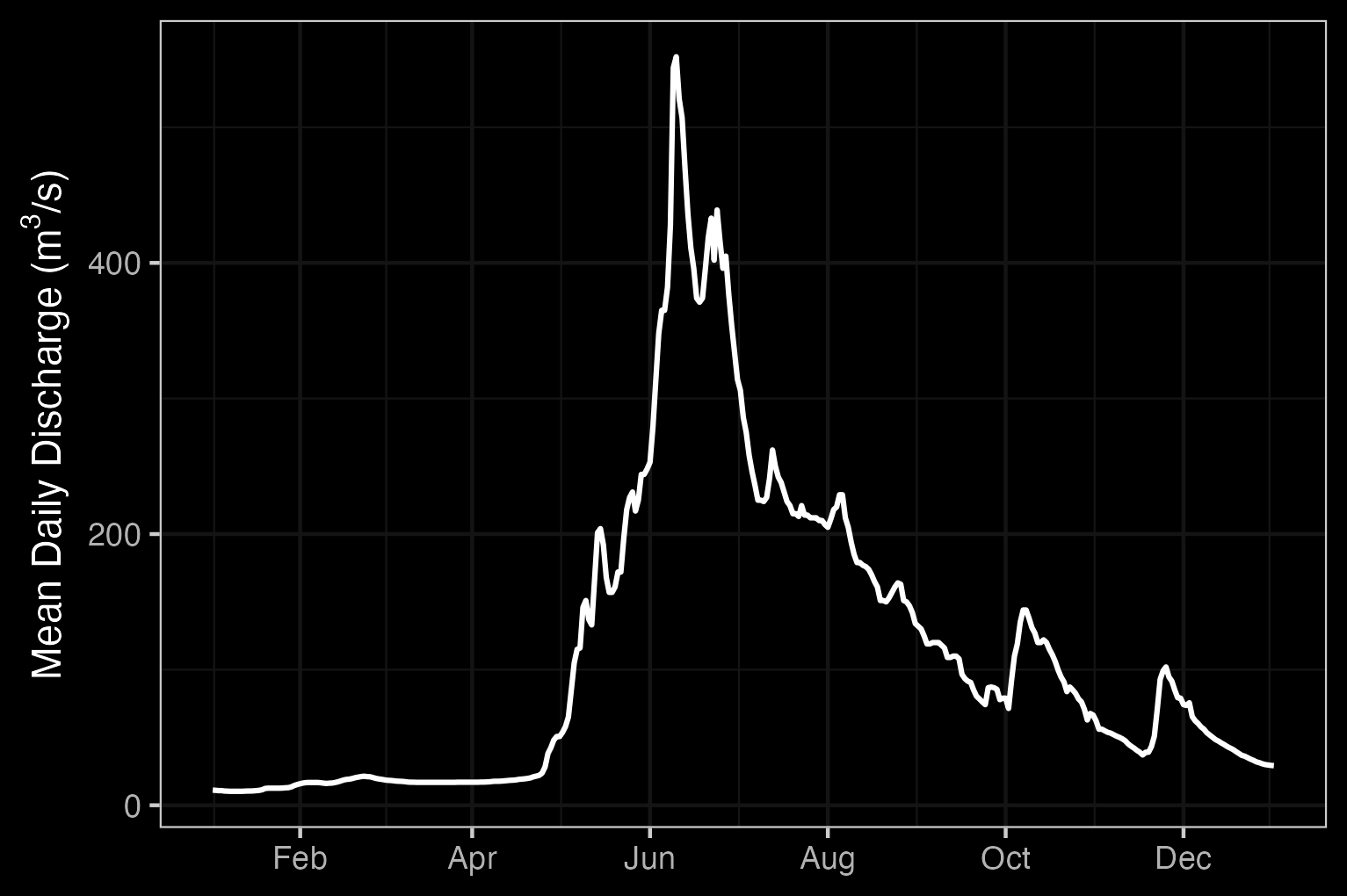
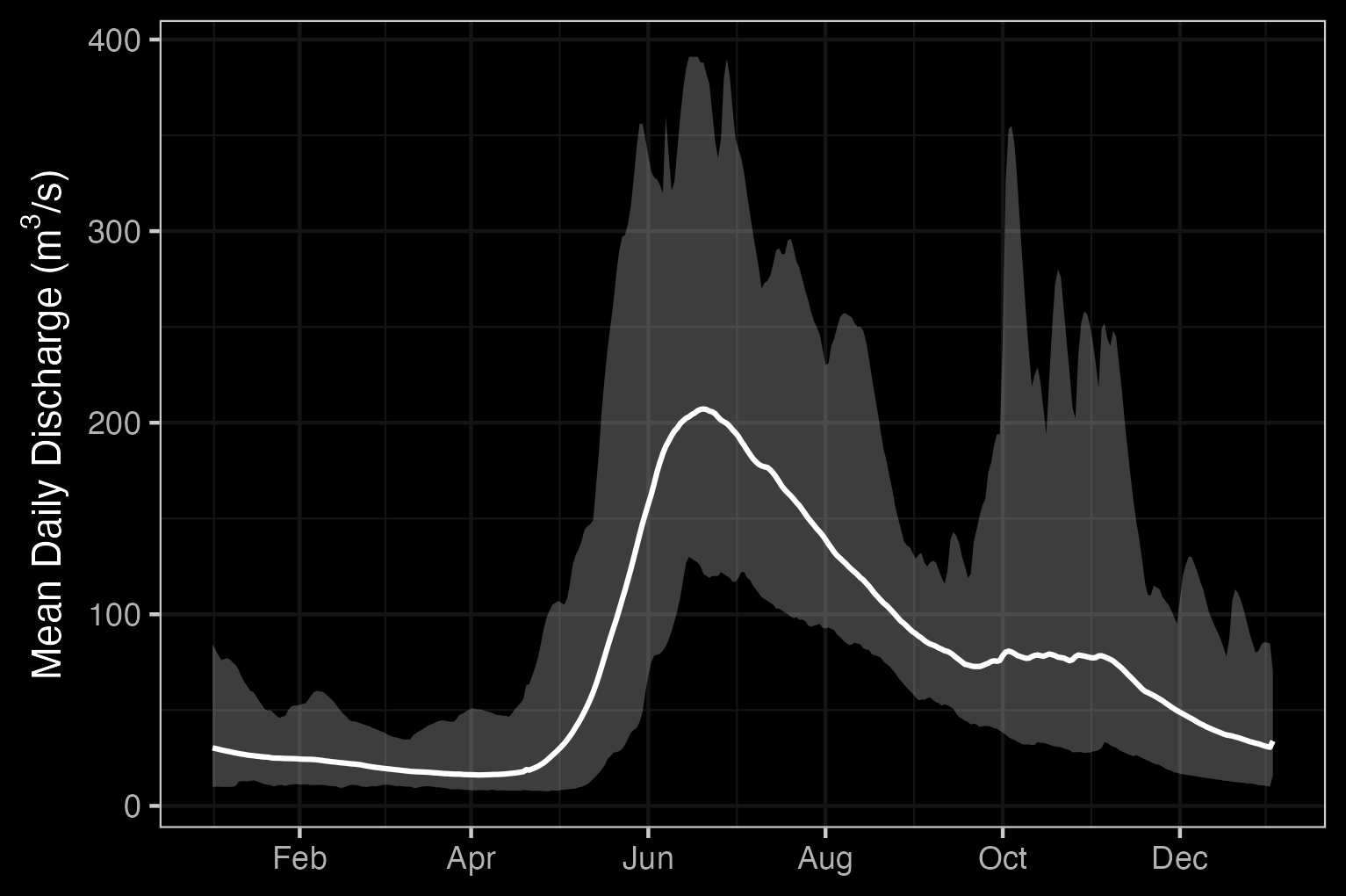
Figure 2.5: Left: Hydrograph for Morice River near Houston (Station #08ED003 - 1971 data only). Right: Hydrograph for Morice River near outlet of Morice Lake (Station #08ED002).
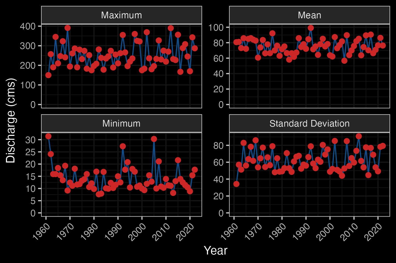
Figure 2.6: Summary of hydrology statistics for Morice River near outlet of Morice Lake (Station #08ED002 - Lat 54.116829 Lon -127.426582). Available daily discharge data from 1961 to 2022.
2.6 Zymoetz River
The Zymoetz River (known locally as the Copper River) watershed is an eighth order stream that drains an area of 3026km2 in a generally westerly direction. It is considered a major tributary of the Skeena River, as it contributes approximately 10% of the flow. The headwater lakes are located approximately 20km southwest of Smithers, and they include Aldrich, Dennis and McDonell Lakes. The upper and lower portions of the watershed are accessed via logging roads off of Highway 16 from Smithers and Terrace, respectively. Access to the middle watershed is difficult due to road wash out. The Zymoetz River flows roughly 120km, starting just west of Hudson Bay mountain near Smithers and ending at the confluence of the Skeena River, approximately 8km north-east of Terrace. Elevations in the watershed range from 120m at the confluence, to 2740m in the Howson Range. The Duthie mine operated on the south-west slope of Hudson Bay Mountain during the 1930’s and 1950’s, and reports have documented contaminated streams and lakes in the surrounding area (Allen Gottesfeld, Rabnett, and Hall 2002). The lower end of the Zymoetz watershed has seen a significant reduction in riparian habitat due to fires, forest development practices, pipe line and road construction (Allen Gottesfeld, Rabnett, and Hall 2002). Snowmelt plays a big role in controlling the stream hydrology, with a mean annual discharge estimated at 106 m3/s at station 08EF005 located near Smithers. Peak discharge happens in May to early June, which is typical of a high elevation watershed like this (Figures 2.7 - 2.8).
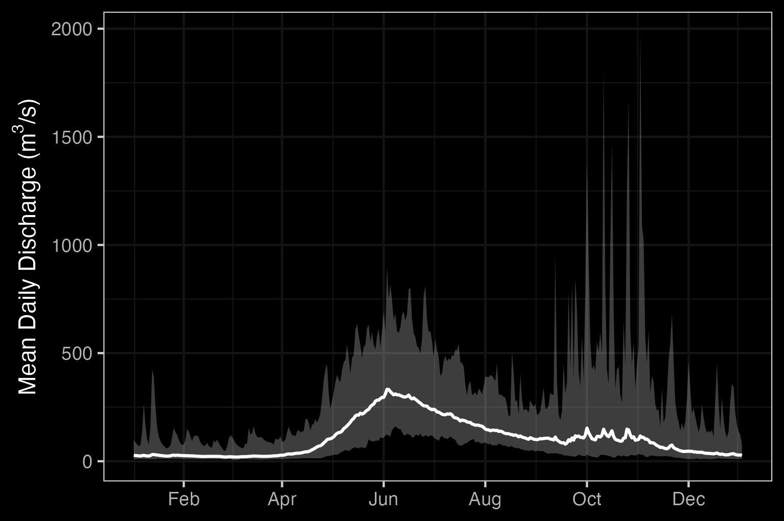
Figure 2.7: Zymoetz River Above O.k. Creek (Station #08EF005 - Lat 54.49363 Lon -128.32466). Available mean daily discharge data from 1963 to 2021.
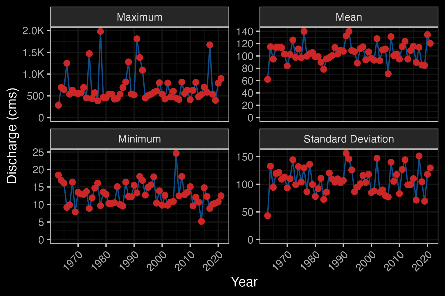
Figure 2.8: Zymoetz River Above O.k. Creek (Station #08EF005 - Lat 54.49363 Lon -128.32466). Available daily discharge data from 1963 to 2021.
2.6.1 Kispiox River
The Kispiox River watershed is a seventh order stream that drains an area of 2100km2 in a south east direction. It is a large tributary of the Skeena River, contributing approximately 9% of its flow. It flows 140km to the confluence of the Skeena River, near Kispiox Village. Elevations in the watershed range from 200m at the mouth to as high as 2090m on Kispiox Mountain. The mainstream of the Kispiox is fed mainly by glacier melt and high elevation snow melt. Swan and Stephens Lakes (located in the upper watershed) are important sockeye systems. Swan Lake drains via Club Lake into Stephens Lake which in turn flows via Stephens Creek into the mainstem of the Kispiox River. Some of the biggest threats to aquatic ecosystems in the Kispiox valley are reported as erosion, obstructions, sedimentation, and altered water yield. The upper third of the Kispiox watershed (upstream of the Nangeese River) is well protected from development by the Swan Lake Kispiox River Provincial Park and because it contains few roads with little forestry development (Allen Gottesfeld, Rabnett, and Hall 2002). The Kispiox River has a mean annual discharge estimated at 45 m3/s at station 08EB004 located near Hazelton. Peak discharge happens in May and June as a result of the spring snowmelt (Figures 2.9 - 2.10).
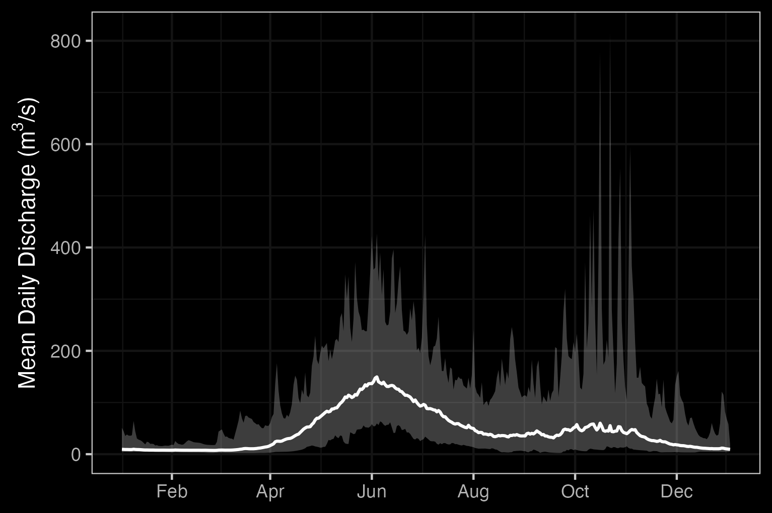
Figure 2.9: Kispiox River Near Hazelton (Station #08EB004 - Lat 55.43385 Lon -127.71616). Available mean daily discharge data from 1963 to 2022.
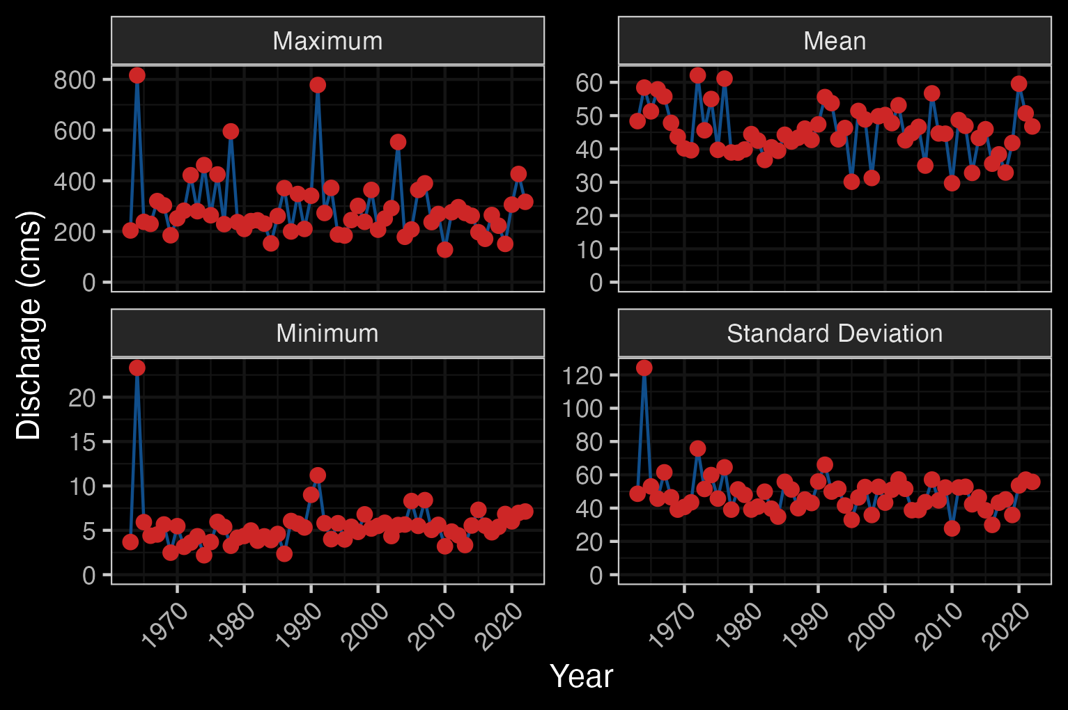
Figure 2.10: Kispiox River Near Hazelton (Station #08EB004 - Lat 55.43385 Lon -127.71616). Available daily discharge data from 1963 to 2022.
2.7 Kitsumkalum River
The Kitsumkalum River is a sixth order stream that flows east from the Coast Mountains to Kitsumkalum lake then south to Terrace where it joins the Skeena River, draining an area of 2289km2. Major tributaries to the Kitsumkalum River include the Cedar River, Nelson River, Mayo Creek, Goat Creek, Lean-To Creek and Deep Creek (McElhanney 2022). Peak flows occur in May-June from snow melt with subsequent peaks the fall from rain events (McElhanney 2022). There is one hydrometric station below Kitsumkalum lake which has been active since 2018, and has a mean annual discharge of round(fasstr::calc_longterm_mean(station_number = "08EG019")$LTMAD,0)m3/s (Figures 2.11 - 2.12. From 1929-1954, there was a hydrometric station near Terrace, which estimated the mean annual discharge to be 138m3/s.
The Kitsumkalum River watershed has been highly impacted by logging. Many of the tributaries to the Kitsumkalum River have altered channel morphology, increased bedload movement, bank failures, sediment loading, and debris accumulation (A. Gottesfeld and Rabnett 2007).
There has been a significant amount of work done to enhance salmon populations within the watershed. The SkeenaWild Conservation Trust is conducting riparian restoration surveys on several tributaries to the Kitsumkalum River, including Willow Creek, Spring Creek, Lean-To Creek, and Deep Creek (Healthy Watersheds Initiative 2021). The Deep Creek Hatchery, operated by the Terrace Salmonid Enhancement Society, has been supporting Kitsumkalum River chinook populations since 1984 (A. Gottesfeld and Rabnett 2007). Additionally, there is a small groundwater facility for the incubation and rearing coho and chum, run by the Kitsumkalum First Nation (A. Gottesfeld and Rabnett 2007). In 2000 The Clear Creek Eastern Side Channel was constructed to enhance juvenile rearing habitat and adult spawning habitat for coho salmon on Clear Creek, a tributary to the Kitsumkalum River, however the site has not been maintained and beaver activity has obstructed fish accessibility to much of the channel (Elmer 2021).
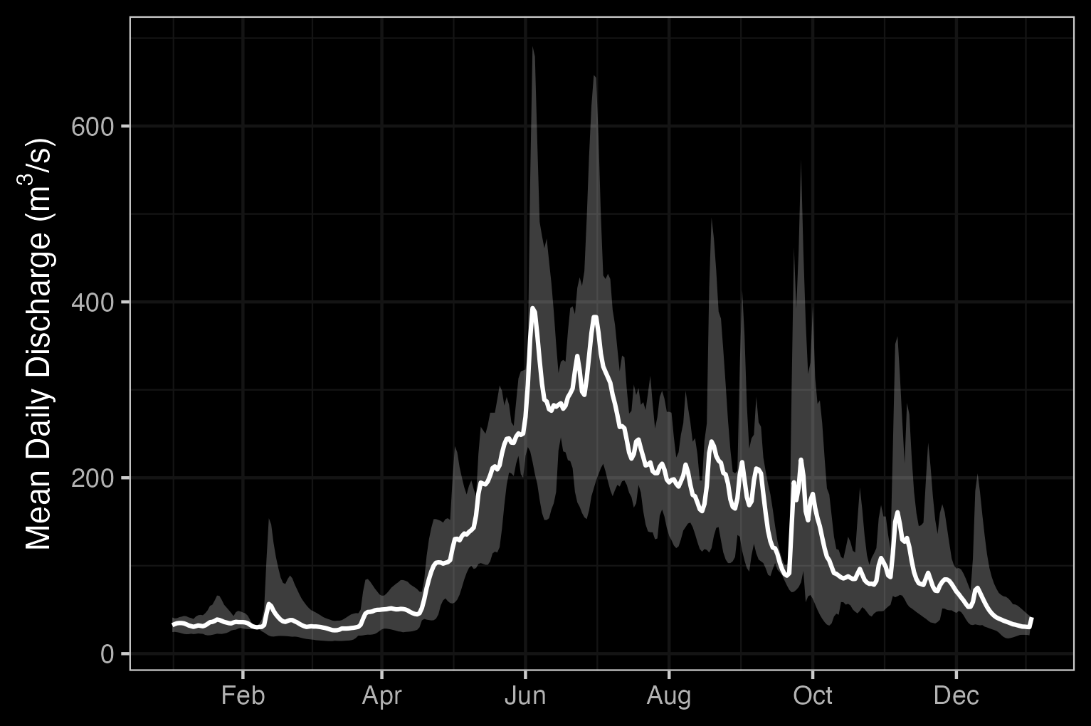
Figure 2.11: Kitsumkalum River Below Alice Creek (Station #08EG019 - Lat 54.6793 Lon -128.74396). Available mean daily discharge data from 2018 to 2022.
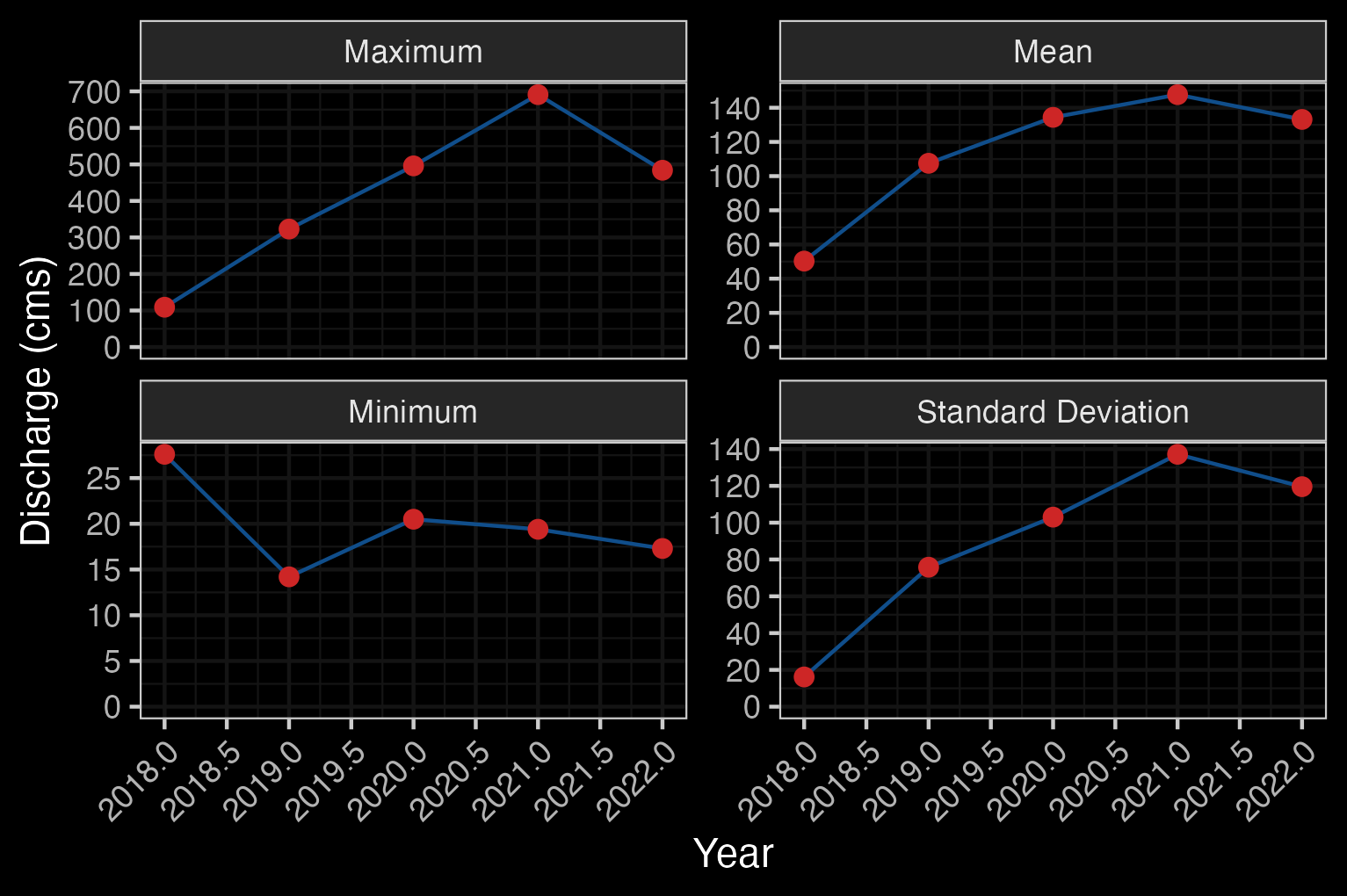
Figure 2.12: Kitsumkalum River Below Alice Creek (Station #08EG019 - Lat 54.6793 Lon -128.74396). Available daily discharge data from 2018 to 2022.
2.8 Fisheries
In 2004, IBM Business Consulting Services (2006) estimated the value of Skeena Fisheries at an annual average of $110 million dollars. The Bulkley-Morice watershed is an integral part of the salmon production in the Skeena drainage and supports an internationally renown steelhead, chinook and coho sport fishery (Tamblyn 2005).
2.8.1 Bulkley River
Traditionally, the salmon stocks passing through and spawning in the greater Bulkley River were the principal food source for the Gitxsan and Wet’suwet’en people living there (Wilson and Rabnett 2007). Anadromous lamprey passing through and spawning in the upper Bulkley River were traditionally also an important food source for the Wet’suwet’en (A. Gottesfeld and Rabnett (2007); pers comm. Mike Ridsdale, Environmental Assessment Coordinator, Office of the Wet’suwet’en). A. Gottesfeld and Rabnett (2007) report sourceing information from Department of Fisheries and Oceans (1991) that principal spawning areas for chinook in the Neexdzii Kwah include the mainstem above and below Buck and McQuarrie Creeks, between Cesford and Watson Creeks, and the reaches upstream and downstream of Bulkley Falls.
Renowned as a world class recreational steelhead and coho fishery, the greater Bulkley River receives some of the heaviest angling pressure in the province. In response to longstanding angler concerns with respect to overcrowding, quality of experience and conflict amongst anglers, an Angling Management Plan was drafted for the river following the initiation of the Skeena Quality Waters Strategy process in 2006 and an extensive multi-year consultation process. The plan introduces a number of regulatory measures with the intent to provide Canadian resident anglers with quality steelhead fishing opportunities. Regulatory measures introduced with the Angling Management Plan include prohibited angling for non-guided non-resident aliens on Saturdays and Sundays, Sept 1 - Oct 31 within the Bulkley River, angling prohibited for non-guided non-resident aliens on Saturdays and Sundays, all year within the Suskwa River and angling prohibited for non-guided non-resident aliens Sept 1 - Oct 31 in the Telkwa River. The Neexdzii Kwah is considered Class II water and there is no fshing permitted upstream of the Morice/Bulkley River Confluence (FLNRO 2013a, 2013b; FLNRORD 2019).
2.8.1.1 Upper Bulkley Falls
A detailed field assessment and write up regarding the upper Bulkley falls was conducted as part of fish passage restoration in the watershed - is presented in Irvine (2021) with a condensed summary here. The site was assessed on October 28, 2021 by Nallas Nikal, B.i.T, and Chad Lewis, Environmental Technician. The top of the falls is located at 11U.678269.6038266 at an elevation of 697m approximatley 11.3km downstream of Bulkley Lake and upstream of Ailport Creek. Within the Bulkley River immediately below the 12 - 15m high bedrock falls, channel width was 17.4m and the wetted width was 15.6m. Two channels comprised the falls. The primary channel was 20m long, had a channel/wetted width of 8.5m, a 16% grade and water depths ranging from 35 - 63cm. The secondary channel was 25m long, with channel/wetted widths of 7.5m, a grade of 12% and water depths ranging from 3 - 13cm (Irvine 2021).
Dyson (1949) and Stokes (1956) report substantial use of habitat above Bulkley Falls by steelhead, chinook, coho and sockeye utilization in the past (pre-1950) based on spawning reports. Both authors concluded that the Bulkley Falls pose a partial obstruction to migrating fish based on flow levels. Chinook, which migrate early in the summer when water levels are high, have been noted as able to ascend the falls in normal to high water years and in high water years it was thought that coho and steelhead could ascend. A. Gottesfeld and Rabnett (2007) report that the falls are almost completely impassable to all salmon during low water flows. Stokes (1956) reports that there was high value spawning habitat located within the first 3km of the Neexdzii Kwah from the outlet of Bulkley Lake.
Wilson and Rabnett (2007) reported that approximately 11.3 km downstream of the Bulkley Lake outlet and just upstream of Watson Creek, the upper Bulkley falls is an approximately 4m high narrow rock sill that crosses the Neexdzii Kwah, producing a steep cascade section. This obstacle to fish passage is recorded as an almost complete barrier to fish passage for salmon during low water flows. Wilson and Rabnett (2007) also reported that coho have not been observed beyond the falls since 1972.
2.8.2 Morice River
Detailed reviews of Morice River watershed fisheries can be found in Bustard and Schell (2002), Allen Gottesfeld, Rabnett, and Hall (2002), Schell (2003), A. Gottesfeld and Rabnett (2007), and ILMB (2007) with a comprehensive review of water quality by Oliver (2018) Overall, the Morice watershed contains high fisheries values as a major producer of chinook, pink, sockeye, coho and steelhead.
2.8.3 Zymoetz River
Within the Zymoetz Watershed, there are many areas with high fishery values. Steelhead are the most extensively documented fish species in the Zymoetz River watershed. Adults enter the river from July to November and then go on to spawn the following year in late spring to early summer. The Zymoetz River is a relatively steep system. Two canyons are located 6.4 and 19.6 kilometers upstream of the Skeena River confluence. These canyons make access to the Zymoetz difficult for pink and chum salmon (Allen Gottesfeld, Rabnett, and Hall 2002). The Zymoetz River is renowned for its aggressive steelhead that have been known to take flies or lures. There is a 50km stretch upstream of Limonite Creek that’s very remote and offers high quality fishing opportunities for anglers (FLNRORD 2013).
Traditional First Nations use of the upper Zymoetz River watershed by the Gitxsan and Wet’suwet’en people differed between community sites, residences, and fish houses, and was large and diverse. From the upper to lower Zymoetz River and to the Skeena River, a significant ancient grease trail connected, with a branch track forking through Limonite Creek and flowing down the Telkwa River. The fishery used a weir at the mouth of McDonell Lake and spears at Six Mile Flats, near Dennis Lake. There is no information on native fisheries on the lower Zymoetz River. The Zymoetz is considered to be one of the top ten steelhead rivers in BC (Allen Gottesfeld, Rabnett, and Hall 2002).
2.8.4 Kispiox River
Kispiox River salmon are a important food source and cultural symbol for the Gitxsan people with sockeye and coho historically the two most significant species. Gitangwalk and Lax Didax, two significant villages that were both abandoned in the early 1900s, were situated on the Kispiox in such a way as to block the sockeye and coho salmon’s upstream migration to the Upper Kispiox River spawning grounds providing opportunities to gather and preserve a significant amount of high-quality food over relatively short time periods (Allen Gottesfeld, Rabnett, and Hall 2002). The 100 km of mainstem and 300km of tributary streams in the Kispiox River Watershed are considering high value fish habitat supporting migration, spawning and rearing for many fish species. The Kispiox fisheries supports both recreational and commercial fishing while also enhancing the ecology, nutrient regime, and structural diversity of the drainage. Since 1992, sockeye and coho escapements from the Kispiox Watershed have been documented by the Gitxsan Watershed Authorities as they creates strong cultural, economic, and symbolic ties for the local communities (Allen Gottesfeld, Rabnett, and Hall 2002).
2.8.5 Kitsumkalum River
The Kitsumkalum River is an important waterway for all species of salmon. It is one of the three main chinook producing rivers in the Skeena watershed and supports all five species of pacific salmon, steelhead, and other resident trout and char species (McElhanney 2022). Most notably, the Kitsumkalum River has consistently produced the largest-bodied chinook in the Skeena Watershed, as well as on most of the Pacific coast (A. Gottesfeld and Rabnett 2007). The watershed supports strong recreational coho, steelhead, and chinook fishing. Kitsumkalum salmon also play an important role in the culture and economy of the Kitsumkalum Band (A. Gottesfeld and Rabnett 2007).
2.8.6 Salmon Stock Assessment Data
Fisheries and Oceans Canada stock assessment data was accessed via the NuSEDS-New Salmon Escapement Database System through the Open Government Portal with results presented in Table 2.1. A brief memo on the data extraction process is available here.
dfo_sad_tr <- readr::read_csv('data/inputs_raw/All Areas NuSEDS.csv') %>%
  dplyr::filter(!is.na(total_return_to_river)) %>%
  arrange(species, analysis_yr) %>%
  dplyr::select(waterbody,
                species, analysis_yr,
                total_return_to_river,
                start_spawn_dt_from,
                peak_spawn_dt_from,
                end_spawn_dt_from,
                accuracy,
                precision,
                index_yn,
                reliability,
                estimate_stage,
                estimate_classification,
                no_inspections_used,
                estimate_method) |>
  janitor::clean_names(case = "title")

dfo_sad_tr |>
  gt::gt() |> # need to make tibble a gt table object
  gt::tab_header(title = "Fisheries and Oceans Canada stock assessment data for the Skeena watershed.  Data can be filtered to specific waterbodies") |>
  mygt()
2.8.7 Fish Species
Fish species recorded in the Morice, Bulkley, Zymoetz, Kispiox, and Kitsumkalum Rivers watershed groups are detailed in Table 2.2 (MoE 2019a). Coastal cutthrout trout and bull trout are considered of special concern (blue-listed) provincially. Summaries of some of the Skeena fish species life history, biology, stock status, and traditional use are documented in Schell (2003), Wilson and Rabnett (2007), Allen Gottesfeld, Rabnett, and Hall (2002) and Office of the Wet’suwet’en (2013). Wilson and Rabnett (2007) discuss chinook, pink, sockeye, coho, steelhead and indigenous freshwater Bulkley River fish stocks within the context of key lower and upper Bulkley River habitats such as the Suskwa River, Station Creek, Harold Price Creek, Telkwa River and Buck Creek. Key areas within the upper Bulkley River watershed with high fishery values, documented in Schell (2003), are the upper Bulkley mainstem, Buck Creek, Dungate Creek, Barren Creek, McQuarrie Creek, Byman Creek, Richfield Creek, Johnny David Creek, Aitken Creek and Emerson Creek.
Some key areas of high fisheries values for chinook, sockeye and coho are noted in Bustard and Schell (2002) as McBride Lake, Nanika Lake, and Morice Lake watersheds. A draft gantt chart for select species in the Morice River and Bulkley River watersheds was derived from reviews of the aforementioned references and is included as Figure 2.13. The data is considered in draft form and will be refined over the spring and summer of 2021 with local fisheries technicians and knowledge holders during the collaboratory assessment planning and fieldwork activities planned.
In the 1990’s the Morice River watershed, A. Gottesfeld and Rabnett (2007) estimated that chinook comprised 30% of the total Skeena system chinook escapements. It is estimated that Morice River coho comprise approximatley 4% of the Skeena escapement with a declining trend noted since the 1950 in A. Gottesfeld and Rabnett (2007). Coho spawn in major tributaries and small streams ideally at locations where downstream dispersal can result in seeding of prime off channel habitats including warm productive sloughs and side channels. Of all the salmon species, coho rely on small tributaries the most (Bustard and Schell 2002). Bustard and Schell (2002) report that much of the distribution of coho into non-natal tributaries occurs during high flow periods of May - early July with road culverts blocking migration into these habitats.
##### Chinook
#  In the 1990's Morice River watershed, @gottesfeld_rabnett2007SkeenaFish estimated that chinook comprised 30% of the total Skeena system chinook escapements. @buckwalter_kirsch2012Fishinventory have recorded juvenile chinook rearing in small non natal streams.

# @buckwalter_kirsch2012Fishinventory have uvenile chinook have been recorded rearing in small non natal streams


#It is estimated that Morice River coho comprise approximatley 4% of the Skeena escapement with a declining trend noted since the 1950 in @gottesfeld_rabnett2007SkeenaFish.  Coho spawn in major tributaries and small streams ideally at locations where downstream dispersal can result in seeding of prime off channel habitats including warm productive sloughs and side channels.  Of all the salmon species, coho rely on small tributaries the most [@bustard_schell2002ConservingMorice]. @bustard_schell2002ConservingMorice report that much of the distribution of coho into non-natal tributaries occurs during high flow periods of May - early July with road culverts blocking migration into these habitats.
Summaries of historical fish observations in the Bulkley River and Morice River watershed groups (n=4033), graphed by remotely sensed average gradient as well as measured or modelled channel width categories for their associated stream segments where calculated with bcfishpass and bcfishobs and are provided in Figures 2.14 - 2.15.
fiss_species_table <- readr::read_csv('data/inputs_extracted/fiss_species_table.csv')

fiss_species_table %>%
  fpr::fpr_kable(caption_text = 'Fish species recorded in the Morice River, Bulkley River, Zymoetz River, Kispiox River, and Kitsumkalum River watershed groups.',
                 footnote_text = 'COSEWIC abbreviations :
                 SC - Special concern
                 DD - Data deficient
                 NAR - Not at risk
                 E - Endangered
                 T - Threatened

                 BC List definitions :
                 Yellow - Species that is apparently secure
                 Blue - Species that is of special concern
                 Exotic - Species that have been moved beyond their natural range as a result of human activity
                 ',
scroll = gitbook_on)| Scientific Name | Species Name | BC List | COSEWIC | Bulkley | Kispiox | Kalum | Morice | Zymoetz |
|---|---|---|---|---|---|---|---|---|
| Catostomus catostomus | Longnose Sucker | Yellow | – | Yes | Yes | – | Yes | Yes |
| Catostomus commersonii | White Sucker | Yellow | – | Yes | Yes | Yes | Yes | – |
| Catostomus macrocheilus | Largescale Sucker | Yellow | – | Yes | Yes | Yes | Yes | Yes |
| Chrosomus eos | Northern Redbelly Dace | Yellow | – | Yes | – | – | – | – |
| Coregonus clupeaformis | Lake Whitefish | Yellow | – | Yes | Yes | – | Yes | – |
| Coregonus sardinella | Least Cisco | Blue | – | – | – | Yes | – | – |
| Cottus aleuticus | Coastrange Sculpin (formerly Aleutian Sculpin) | Yellow | – | Yes | Yes | Yes | Yes | – |
| Cottus asper | Prickly Sculpin | Yellow | – | Yes | Yes | Yes | Yes | Yes |
| Cottus cognatus | Slimy Sculpin | Yellow | – | – | Yes | Yes | – | – |
| Couesius plumbeus | Lake Chub | Yellow | DD | Yes | Yes | Yes | Yes | – |
| Entosphenus tridentatus | Pacific Lamprey | Yellow | – | Yes | – | Yes | Yes | – |
| Gasterosteus aculeatus | Threespine Stickleback | Yellow | – | – | Yes | Yes | – | – |
| Hybognathus hankinsoni | Brassy Minnow | No Status | – | Yes | – | – | – | – |
| Lampetra ayresii | River Lamprey | Yellow | – | – | – | Yes | – | – |
| Lota lota | Burbot | Yellow | – | Yes | Yes | Yes | Yes | Yes |
| Mylocheilus caurinus | Peamouth Chub | Yellow | – | Yes | Yes | Yes | Yes | Yes |
| Oncorhynchus clarkii | Cutthroat Trout | No Status | – | Yes | Yes | Yes | Yes | Yes |
| Oncorhynchus clarkii | Cutthroat Trout (Anadromous) | No Status | – | Yes | Yes | – | – | Yes |
| Oncorhynchus clarkii clarkii | Coastal Cutthroat Trout | Blue | – | Yes | Yes | Yes | Yes | Yes |
| Oncorhynchus clarkii lewisi | Westslope (Yellowstone) Cutthroat Trout | Blue | SC (Nov 2016) | – | Yes | Yes | – | – |
| Oncorhynchus gorbuscha | Pink Salmon | Yellow | – | Yes | Yes | Yes | Yes | Yes |
| Oncorhynchus keta | Chum Salmon | Yellow | – | Yes | Yes | Yes | Yes | Yes |
| Oncorhynchus kisutch | Coho Salmon | Yellow | – | Yes | Yes | Yes | Yes | Yes |
| Oncorhynchus mykiss | Rainbow Trout | Yellow | – | Yes | Yes | Yes | Yes | Yes |
| Oncorhynchus mykiss | Steelhead | Yellow | – | Yes | Yes | Yes | Yes | Yes |
| Oncorhynchus mykiss | Steelhead (Summer-run) | Yellow | – | Yes | – | – | Yes | – |
| Oncorhynchus mykiss | Steelhead (Winter-run) | Yellow | – | – | Yes | – | – | Yes |
| Oncorhynchus nerka | Kokanee | Yellow | – | Yes | Yes | Yes | Yes | Yes |
| Oncorhynchus nerka | Sockeye Salmon | Yellow | – | Yes | Yes | Yes | Yes | Yes |
| Oncorhynchus tshawytscha | Chinook Salmon | Yellow | E/T/SC (Dec 2018) | Yes | Yes | Yes | Yes | Yes |
| Prosopium coulterii | Pygmy Whitefish | Yellow | NAR (Nov 2016) | Yes | Yes | – | Yes | – |
| Prosopium coulterii pop. 3 | Giant Pygmy Whitefish | Yellow | – | Yes | – | – | – | – |
| Prosopium cylindraceum | Round Whitefish | Yellow | – | – | – | Yes | – | – |
| Prosopium williamsoni | Mountain Whitefish | Yellow | – | Yes | Yes | Yes | Yes | Yes |
| Ptychocheilus oregonensis | Northern Pikeminnow | Yellow | – | Yes | Yes | – | Yes | Yes |
| Pungitius pungitius | Ninespine Stickleback | Unknown | – | Yes | – | – | – | – |
| Rhinichthys cataractae | Longnose Dace | Yellow | – | Yes | Yes | Yes | Yes | Yes |
| Rhinichthys falcatus | Leopard Dace | Yellow | NAR (May 1990) | – | – | – | Yes | – |
| Richardsonius balteatus | Redside Shiner | Yellow | – | Yes | Yes | Yes | Yes | Yes |
| Salvelinus confluentus | Bull Trout | Blue | SC (Nov 2012) | Yes | Yes | Yes | Yes | Yes |
| Salvelinus fontinalis | Brook Trout | Exotic | – | Yes | – | – | Yes | – |
| Salvelinus malma | Dolly Varden | Yellow | – | Yes | Yes | Yes | Yes | Yes |
| Salvelinus namaycush | Lake Trout | Yellow | – | Yes | Yes | – | Yes | – |
| – | All Salmon | – | – | – | Yes | Yes | – | – |
| – | Arctic Char | – | – | – | – | – | Yes | – |
| – | Chub (General) | – | – | – | Yes | – | – | – |
| – | Cutthroat/Rainbow cross | – | – | Yes | Yes | Yes | – | – |
| – | Dace (General) | – | – | – | – | – | Yes | – |
| – | Lamprey (General) | – | – | Yes | Yes | Yes | Yes | – |
| – | Minnow (General) | – | – | Yes | Yes | – | Yes | – |
| – | Mottled Sculpin | – | – | Yes | – | – | – | – |
| – | Salmon (General) | – | – | Yes | Yes | – | Yes | Yes |
| – | Sculpin (General) | – | – | Yes | Yes | Yes | Yes | Yes |
| – | Squanga | – | – | – | Yes | – | – | – |
| – | Stickleback (General) | – | – | – | Yes | Yes | – | – |
| – | Sucker (General) | – | – | Yes | Yes | Yes | Yes | Yes |
| – | Verified DV BT hybrid | – | – | – | – | Yes | – | – |
| – | Whitefish (General) | – | – | Yes | Yes | Yes | Yes | Yes |
|
* COSEWIC abbreviations : SC - Special concern DD - Data deficient NAR - Not at risk E - Endangered T - Threatened BC List definitions : Yellow - Species that is apparently secure Blue - Species that is of special concern Exotic - Species that have been moved beyond their natural range as a result of human activity |
gantt_raw <- read_csv("data/inputs_raw/fish_species_life_history_gantt.csv")


##start with just the morice to keep it simple
# ungroup()
##start with just the morice to keep it simple
gantt <- gantt_raw %>%
  select(Species,
         life_stage,
         morice_start2,
         morice_end2) %>%
  filter(
    life_stage != 'Rearing' &
      life_stage != 'Upstream fry migration' &
      !is.na(life_stage),
    !is.na(morice_start2)
  )%>%
  mutate(
    morice_start2 = lubridate::as_date(morice_start2),
    morice_end2 = lubridate::as_date(morice_end2),
    life_stage = factor(life_stage, levels =
                          c('Migration', 'Overwintering', 'Spawning', 'Incubation', 'Emergence', 'Outmigration')),
    life_stage = forcats::fct_rev(life_stage) ##last line was upside down!
  ) %>%
  filter(life_stage != 'Overwintering')


##make a plot
ggplot(gantt, aes(xmin = morice_start2,
                  xmax = morice_end2,
                  y = life_stage,
                  color = life_stage)) +
  geom_linerange(size = 2) +
  labs(x=NULL, y=NULL)+
  # theme_bw()+
  ggdark::dark_theme_bw(base_size = 11)+
  theme(legend.position = "none")+
  scale_x_date(date_labels = "%B")+
  facet_wrap(~Species, ncol = 1)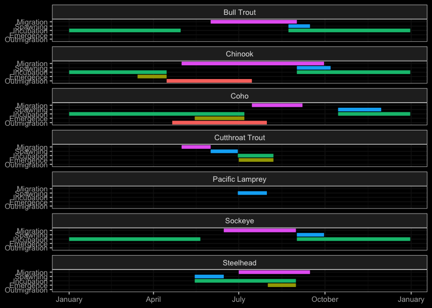
Figure 2.13: Gantt chart for select species in the Morice River and Bulkley River watersheds. To be updated in consultation with local fisheries techicians and knowledge holders.
# fiss_sum <- readr::read_csv(file = paste0(getwd(), '/data/extracted_inputs/fiss_sum.csv'))
fiss_sum_grad <- readr::read_csv(file = 'data/inputs_extracted/fiss_sum_grad.csv')
fiss_sum_width <- readr::read_csv(file = 'data/inputs_extracted/fiss_sum_width.csv')

# A summary of historical westslope cutthrout trout observations in the Elk River watershed group by average gradient category of associated stream segment is provided in Figure \@ref(fig:fish-wct-bar). Of `r wct_elkr_grad %>% filter(gradient_id == 3) %>% pull(total)` observations, `r wct_elkr_grad %>% filter(gradient_id == 3) %>% pull(Percent) + wct_elkr_grad %>% filter(gradient_id == 5) %>% pull(Percent) + wct_elkr_grad %>% filter(gradient_id == 8) %>% pull(Percent)`% were within stream segments with average gradients ranging from 0 - 8%.  A total of `r wct_elkr_grad %>% filter(gradient_id == 3) %>% pull(Percent)`% of historic observations were within stream segments with gradients between 0 - 3%, `r wct_elkr_grad %>% filter(gradient_id == 5) %>% pull(Percent)`% were within stream segments with gradients ranging from 3 - 5% and `r wct_elkr_grad %>% filter(gradient_id == 5) %>% pull(Percent)`% were within stream segments with gradients between 5 - 8% [@data_fish_obs; @norris2020bcfishobs].
##bar graph
plot_grad <- fiss_sum_grad %>%
filter(gradient_id != 99) %>%
ggplot(aes(x = Gradient, y = Percent)) +
geom_bar(stat = "identity")+
facet_wrap(~species_code, ncol = 2)+
ggdark::dark_theme_bw(base_size = 11)+
labs(x = "Average Stream Gradient", y = "Occurrences (%)")
plot_grad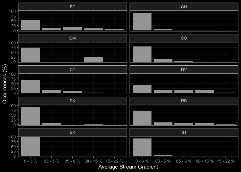
Figure 2.14: Summary of historic salmonid observations vs. stream gradient category for the Bulkley River watershed group.
##bar graph
plot_width <- fiss_sum_width %>%
  filter(!is.na(width_id)) %>%
  ggplot(aes(x = Width, y = Percent)) +
  geom_bar(stat = "identity")+
  facet_wrap(~species_code, ncol = 2)+
  ggdark::dark_theme_bw(base_size = 11)+
  labs(x = "Channel Width", y = "Occurrences (%)")
plot_width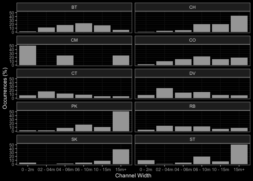
Figure 2.15: Summary of historic salmonid observations vs. channel width category for the Bulkley River watershed group.
##bar graph
fiss_sum_wshed_filter <- fiss_sum %>%
  filter(upstream_area_ha < 5000) %>%
  mutate(upstream_area_km = upstream_area_ha/100)

bin_1 <- 0
# bin_1 <- floor(min(fiss_sum_wshed_filter$upstream_area_ha, na.rm = TRUE)/5)*5
bin_n <- ceiling(max(fiss_sum_wshed_filter$upstream_area_km, na.rm = TRUE)/5)*5
bins <- seq(bin_1,bin_n, by = 5)

plot_wshed_hist <- ggplot(fiss_sum_wshed_filter, aes(x=upstream_area_km
                                           # fill=alias_local_name
                                           # color = alias_local_name
)) +
  geom_histogram(breaks = bins,
                 position="identity", size = 0.75)+
  labs(x = "Upstream Watershed Area (km)", y = "Count Fish (#)") +
  facet_wrap(~species_code, ncol = 2)+
  # scale_color_grey() +
  # scale_fill_grey() +
  ggdark::dark_theme_bw(base_size = 11)+
  scale_x_continuous(breaks = bins[seq(1, length(bins), by = 2)])+
  # scale_color_manual(values=c("grey90", "grey60", "grey30", "grey0"))+
  # theme(axis.text.x = element_text(angle = 45, hjust = 1))+
  geom_histogram(aes(y=..density..), breaks = bins, alpha=0.5,
                 position="identity", size = 0.75)
plot_wshed_hist
## Fish Passage Restoration Planning and Implementation
# As a result of high-level direction from the provincial government, a Fish Passage Strategic Approach protocol has been developed for British Columbia to ensure that the greatest opportunities for restoration of fish passage are pursued. A Fish Passage Technical Working Group has been formed to coordinate the protocol and data is continuously amalgamated within the Provincial Steam Crossing Inventory System (PSCIS). The strategic approach protocol involves a four-phase process as described in @fishpassagetechnicalworkinggroupFishPassageStrategic2014 :
#
# - Phase 1: Fish Passage Assessment -- Fish stream crossings within watersheds with high fish values are assessed to determine barrier status of structures and document a general assessment of adjacent habitat quality and quantity.
# - Phase 2: Habitat Confirmation -- Assessments of crossings prioritized for follow up in Phase 1 studies are conducted to confirm quality and quantity of habitat upstream and down as well as to scope for other potential nearby barriers that could affect the practicality of remediation.
# - Phase 3: Design -- Site plans and designs are drawn for priority crossings where high value fish habitat has been confirmed.
# - Phase 4: Remediation -- Re-connection of isolated habitats through replacement, rehabilitation or removal of prioritized crossing structure barriers.##`r pscis_historic_phase1 %>% filter(watershed_group_code %ilike% 'BULK' & assessment_date < '2020-01-01') %>% nrow()`
### Bulkley River
# There is a rich history of fish passage restoration planning in the Bulkley River watershed group with not all the work documented in the PSCIS system. A non-exhaustive list of historic fish passage reports for the watershed includes @wilson_rabnett2007FishPassage, @mccarthy_fernando20152015Inventory,@smith2018AssessingBarriers @casselman_stanley2010BulkleyFulton and @irvine2018AnalysisPriority.
#
# <br>
#
# Review of the PSCIS database indicated that prior to 2021, 1665 assessments for fish passage (Phase 1) at crossing structures within the Bulkley River watershed group have been recorded in the PSCIS database [@moe2021PSCISAssessments]. No habitat confirmations are recorded in the PSCIS database [@moe2021PSCISHabitat]. Within the Bulkley River watershed group, a number of remediation projects have been completed over the years with backwatering works conducted on Toboggan Creek, Coffin Creek, Moan Creek, Johnny David Creek and potentially others. Three culvert replacements (with open bottom structures) in the watershed group have been tracked in PSCIS and include works on Barren Creek as well as two tributaries to Harold Prince Creek [@moe2021PSCISRemediation]. McDowell Creek at Highway 16 was replaced with a horizontally drilled baffled structure in 2017 and a design is currently being drafted for the Highway 16 crossing over Taman Creek (pers. comm. Kathryn Graham, Regional Manager Environmental Services - Ministry of Transportation and Infrastructure).
#
# ## Morice river
#
# Within the Morice River watershed group prior to 2021, 21 fish passage assessments (Phase 1) had been recorded in the PSCIS database [@moe2021PSCISAssessments]. At the time of reporting, no habitat confirmations had been recorded [@moe2021PSCISHabitat]. Two culvert replacements (with open bottom structures) in the watershed group have been tracked in PSCIS in the and include works on a tributary to the Morice River located at km 39.2 of the Morice River FSR and on bridge installation at km 4 of McBride Road on a tributary to McBride Lake [@moe2021PSCISRemediation].