4 Results and Discussion
Results of Phase 1 and Phase 2 assessments are summarized in Figure 4.1 with additional details provided in sections below.
##make colors for the priorities
pal <-
   colorFactor(palette = c("red", "yellow", "grey", "black"),
               levels = c("high", "moderate", "low", "no fix"))

pal_phase1 <-
   colorFactor(palette = c("red", "yellow", "grey", "black"),
               levels = c("high", "moderate", "low", NA))

# tab_map_phase2 <- tab_map %>% filter(source %like% 'phase2')
#https://stackoverflow.com/questions/61026700/bring-a-group-of-markers-to-front-in-leaflet
# marker_options <- markerOptions(
#   zIndexOffset = 1000)
tracks <- sf::read_sf("./data/habitat_confirmation_tracks.gpx", layer = "tracks")


wshd_study_areas <- sf::read_sf('data/fishpass_mapping/wshd_study_areas.geojson')
  # st_transform(crs = 4326)


map <- leaflet(height=500, width=780) %>%
  addTiles()  %>%
  # leafem::addMouseCoordinates(proj4 = 26911) %>% ##can't seem to get it to render utms yet
  # addProviderTiles(providers$"Esri.DeLorme") %>%
  addProviderTiles("Esri.WorldTopoMap", group = "Topo") %>%
  addProviderTiles("Esri.WorldImagery", group = "ESRI Aerial") %>%
  addPolygons(data = wshd_study_areas, color = "#F29A6E", weight = 1, smoothFactor = 0.5,
              opacity = 1.0, fillOpacity = 0,
              fillColor = "#F29A6E", label = wshd_study_areas$watershed_group_name) %>%
  addPolygons(data = wshds, color = "#0859C6", weight = 1, smoothFactor = 0.5,
              opacity = 1.0, fillOpacity = 0.25,
              fillColor = "#00DBFF",
              label = wshds$stream_crossing_id,
              popup = leafpop::popupTable(x = select(wshds %>% st_set_geometry(NULL),
                                                     Site = stream_crossing_id,
                                                     elev_min:area_km),
                                          feature.id = F,
                                          row.numbers = F),
              group = "Phase 2") %>%
  addLegend(
    position = "topright",
    colors = c("red", "yellow", "grey", "black"),
    labels = c("High", "Moderate", "Low", 'No fix'), opacity = 1,
    title = "Fish Passage Priorities") %>%

addCircleMarkers(data=tab_map %>%
                   filter(source %like% 'phase1' | source %like% 'pscis_reassessments'),
                 label = tab_map %>% filter(source %like% 'phase1' | source %like% 'pscis_reassessments') %>% pull(pscis_crossing_id),
                 # label = tab_map$pscis_crossing_id,
                 labelOptions = labelOptions(noHide = F, textOnly = TRUE),
                 popup = leafpop::popupTable(x = select((tab_map %>% st_set_geometry(NULL) %>% filter(source %like% 'phase1' | source %like% 'pscis_reassessments')),
                                                        Site = pscis_crossing_id, Priority = priority_phase1, Stream = stream_name, Road = road_name, `Habitat value`= habitat_value, `Barrier Result` = barrier_result, `Culvert data` = data_link, `Culvert photos` = photo_link, `Model data` = model_link),
                                             feature.id = F,
                                             row.numbers = F),
                 radius = 9,
                 fillColor = ~pal_phase1(priority_phase1),
                 color= "#ffffff",
                 stroke = TRUE,
                 fillOpacity = 1.0,
                 weight = 2,
                 opacity = 1.0,
                 group = "Phase 1") %>%
  addPolylines(data=tracks,
               opacity=0.75, color = '#e216c4',
               fillOpacity = 0.75, weight=5, group = "Phase 2") %>%

addAwesomeMarkers(
    lng = as.numeric(photo_metadata$gps_longitude),
    lat = as.numeric(photo_metadata$gps_latitude),
    popup = leafpop::popupImage(photo_metadata$url, src = "remote"),
    clusterOptions = markerClusterOptions(),
    group = "Phase 2") %>%

  #commented out this section for now until tab_hab_map object is built from cost estimate table
  addCircleMarkers(
    data=tab_hab_map,
    label = tab_hab_map$pscis_crossing_id,
    labelOptions = labelOptions(noHide = T, textOnly = TRUE),
    popup = leafpop::popupTable(x = select((tab_hab_map %>% st_drop_geometry()),
                                           Site = pscis_crossing_id,
                                           Priority = priority,
                                           Stream = stream_name,
                                           Road = road_name,
                                           `Habitat (m)`= upstream_habitat_length_m,
                                           Comments = comments,
                                           `Culvert data` = data_link,
                                           `Culvert photos` = photo_link,
                                           `Model data` = model_link),
                                feature.id = F,
                                row.numbers = F),
    radius = 9,
    fillColor = ~pal(priority),
    color= "#ffffff",
    stroke = TRUE,
    fillOpacity = 1.0,
    weight = 2,
    opacity = 1.0,
    group = "Phase 2"
    ) %>%

  addLayersControl(
    baseGroups = c(
      "Esri.DeLorme",
      "ESRI Aerial"),
    overlayGroups = c("Phase 1", "Phase 2"),
    options = layersControlOptions(collapsed = F)) %>%
  leaflet.extras::addFullscreenControl() %>%
  addMiniMap(tiles = providers$"Esri.NatGeoWorldMap",
             zoomLevelOffset = -6, width = 100, height = 100)

map %>%
  hideGroup(c("Phase 1"))
Figure 4.1: Map of fish passage and habitat confirmation results
4.1 Fish Passage Assessment - Phase 1
Field assessments were conducted between September 05 2022 and September 26 2022 by Allan Irvine, R.P.Bio. and Mateo Winterscheidt, B.Sc., Tieasha Pierre, Vern Joseph, Dallas Nikal, Alexandria Nikal, Jesse Olson and Colin Morrison. A total of 61 Phase 1 assessments at sites not yet inventoried into the PSCIS system included 18 crossings considered “passable”, 7 crossings considered “potential” barriers and 32 crossings considered “barriers” according to threshold values based on culvert embedment, outlet drop, slope, diameter (relative to channel size) and length (MoE 2011a). Additionally, although all were considered fully passable, 4 crossings assessed were fords and ranked as “unknown” according to the provincial protocol. A summary of crossings assessed, a cost estimate for remediation and a priority ranking for follow up for Phase 1 sites is presented in Table 4.1. Detailed data with photos are presented in Appendix - Phase 1 Fish Passage Assessment Data and Photos.
“Barrier” and “Potential Barrier” rankings used in this project followed MoE (2011a) and reflect an assessment of passability for juvenile salmon or small resident rainbow trout at any flows potentially present throughout the year (Clarkin et al. 2005 ; Bell 1991; Thompson 2013). As noted in Bourne et al. (2011), with a detailed review of different criteria in Kemp and O’Hanley (2010), passability of barriers can be quantified in many different ways. Fish physiology (i.e. species, length, swim speeds) can make defining passability complex but with important implications for evaluating connectivity and prioritizing remediation candidates (Bourne et al. 2011; Shaw et al. 2016; Mahlum et al. 2014; Kemp and O’Hanley 2010). Washington Department of Fish & Wildlife (2009) present criteria for assigning passability scores to culverts that have already been assessed as barriers in coarser level assessments. These passability scores provide additional information to feed into decision making processes related to the prioritization of remediation site candidates and have potential for application in British Columbia.
 tab_cost_est_phase1 %>%
  select(`PSCIS ID`:`Cost Est ( $K)`) %>%
   fpr::fpr_kable(caption_text = 'Upstream habitat estimates and cost benefit analysis for Phase 1 assessments conducted on sites not yet inventoried in PSCIS. Steelhead network model (total length stream network <20% gradient).',
scroll = gitbook_on)| PSCIS ID | External ID | Stream | Road | Result | Habitat value | Stream Width (m) | Priority | Fix | Cost Est ( $K) |
|---|---|---|---|---|---|---|---|---|---|
| 2880 | – | Mooluck Creek | Kuldo FSR | Barrier | Medium | 3.50 | mod | SS-CBS | 50 |
| 8525 | – | Tributary to Coal Creek | McDonell FSR | Barrier | Medium | 1.40 | mod | SS-CBS | 50 |
| 8527 | – | Tributary to Zymoetz River | McDonell FSR | Barrier | Low | 1.50 | low | SS-CBS | 50 |
| 196441 | – | Cullon Creek | Kuldo FSR | Potential | High | 3.00 | mod | OBS | 300 |
| 198182 | 8302064 | Tributary to Kispiox River | Helen Lake Rd | Barrier | Medium | 1.40 | mod | SS-CBS | 50 |
| 198183 | 8302070 | Tributary to Kispiox River | Helen Lake Rd | Barrier | Medium | 2.30 | mod | OBS | 300 |
| 198184 | 8302074 | Tributary to Kispiox River | Helen Lake Rd | Barrier | Low | 1.10 | low | SS-CBS | 50 |
| 198185 | 8300115 | Trib to McCully Creek | Helen Lake Rd | Barrier | Low | 1.30 | low | SS-CBS | 200 |
| 198186 | 8300162 | Tributary to Kispiox River | Poplar Park Rd | Potential | Low | 1.20 | low | SS-CBS | 200 |
| 198187 | 2798180 | Tributary to Kispiox River | Poplar Park Rd | Barrier | Low | 2.10 | low | OBS | – |
| 198188 | 8300161 | Tributary to Kispiox River | Poplar Park Rd | Barrier | Low | 2.30 | low | OBS | 1000 |
| 198190 | 8302683 | Sweetie River | Nangeese FSR | Barrier | Low | 1.90 | low | SS-CBS | 50 |
| 198191 | 8302061 | Tributary to Kispiox River | Corral Main | Barrier | Medium | 1.50 | mod | SS-CBS | 50 |
| 198192 | 8302062 | Tributary to Kispiox River | Corral Main | Barrier | Low | 1.90 | low | SS-CBS | 50 |
| 198193 | 8301747 | Tributary to Cullon Creek | Kuldo FSR | Barrier | Low | 1.80 | low | SS-CBS | 50 |
| 198194 | 8301750 | Tributary to Cullon Creek | Kuldo FSR | Barrier | Medium | 1.90 | mod | SS-CBS | 50 |
| 198195 | 8301761 | Tributary to Cullon Creek | Kuldo FSR | Barrier | Low | 1.50 | low | SS-CBS | 50 |
| 198196 | 8300186 | Tributary to Kispiox River | Kispiox Westside Rd | Barrier | Low | 2.40 | low | OBS | 1000 |
| 198197 | 8300105 | Tributary to Kispiox River | Kispiox Valley Rd | Barrier | Low | 1.80 | low | SS-CBS | 200 |
| 198198 | 8300104 | Tributary to Kispiox River | Kispiox Valley Rd | Potential | Low | 1.20 | low | SS-CBS | 200 |
| 198199 | 8300103 | Tributary to Kispiox River | Kispiox Valley Rd | Barrier | Low | 1.40 | low | SS-CBS | 200 |
| 198202 | 8300188 | Tributary to Kitwanga River | Hwy 37 | Potential | Low | 1.80 | low | SS-CBS | 50 |
| 198203 | 2022090901 | Tributary to Kitwanga River | Kitwancool Branch 2 FSR | Potential | Medium | 1.70 | low | SS-CBS | 50 |
| 198204 | 8302421 | Tributary to Kispiox River | Helen 9000 | Potential | Low | 15.00 | low | OBS | 600 |
| 198205 | 8302065 | Tributary to Kispiox River | Helen Lake Rd | Barrier | Low | 2.20 | low | OBS | 300 |
| 198206 | 8300118 | Tributary to McCully Creek | Helen Lake Rd | Barrier | Low | 2.00 | low | OBS | – |
| 198207 | 2022090501 | Tributary to Kispiox River | Poplar Park Rd | Barrier | High | 2.20 | high | OBS | – |
| 198208 | 8300030 | Tributary to Sweetin River | Kispiox Valley Rd | Barrier | Low | 0.80 | low | SS-CBS | 200 |
| 198209 | 8300111 | Tributary to Kispiox River | Kispiox Valley Rd | Barrier | Low | 1.90 | low | SS-CBS | 200 |
| 198210 | 8302403 | Tributary to Kispiox River | Mitten Mainline | Potential | Low | 4.30 | low | OBS | 300 |
| 198213 | 8301749 | Tributary to Cullon Creek | Kuldo FSR | Barrier | Low | 1.00 | low | SS-CBS | 50 |
| 198214 | 8301748 | Tributary to Cullon Creek | Kuldo FSR | Barrier | Low | 1.60 | low | SS-CBS | 50 |
| 198215 | 8300042 | Tributary to Kispiox River | Kispiox Westside Rd | Barrier | High | 5.30 | high | OBS | 1750 |
| 198217 | 8301485 | Tributary to Skeena River | Sik e Dakh Water Tower Rd | Barrier | High | 5.60 | high | OBS | 300 |
| 198218 | 2787053 | Tributary to Kispiox River | Kispiox Valley Rd | Barrier | Medium | 2.00 | mod | OBS | – |
| 198219 | 8300033 | Tributary to Kispiox River | Seventeen Mile Rd | Potential | Medium | 2.50 | low | OBS | 1000 |
| 198220 | 8300095 | Tributary to Kitwanga River | Hwy 37 | Barrier | High | 5.00 | high | OBS | 22875 |
| 198221 | 8300178 | Tributary to Kitwanga River | 11A Ave | Barrier | Medium | 4.00 | mod | OBS | – |
| 198222 | 8302257 | Pinenut Creek | Babine Slide FSR | Barrier | High | 8.20 | high | OBS | 390 |
| 198224 | 4601067 | Tributary to Zymoetz River | Hankin FSR | Barrier | Medium | 1.45 | mod | SS-CBS | 50 |
| 198225 | 8300128 | Sterritt creek | Babine Slide FSR | Barrier | Low | 3.70 | low | OBS | 390 |
| 198230 | 8300108 | Trib to Sammon Lake | Kispiox Valley Rd | Barrier | Medium | 1.90 | mod | SS-CBS | 200 |
| 198236 | 8301994 | Tributary to Kitwanga River | Kitwancool Branch 2 FSR | Barrier | High | 2.30 | high | OBS | 300 |
4.2 Habitat Confirmation - Phase 2
During 2022 field assessments, habitat confirmation assessments were conducted at 8 sites in the Morice River, Zymoetz River and Kispiox River watersheds. A total of approximately 7km of stream was assessed, fish sampling utilizing electrofishing surveys were conducted at two streams. Georeferenced field maps are presented in Attachment 1.
As collaborative decision making was ongoing at the time of reporting, site prioritization can be considered preliminary. In total, 5 crossings were rated as high priorities for proceeding to design for replacement, 2 crossings were rated as moderate priorities, and 0 crossings were rated as low priorities. Results are summarized in Figure 4.1 - 4.4 and Tables 4.2 - 4.6 with raw habitat and fish sampling data included in digital format here. A summary of preliminary modelling results illustrating the quantity of chinook, coho and steelhead spawning and rearing habitat potentially available upstream of each crossing as estimated by measured/modelled channel width and upstream accessible stream length are presented in Figure 4.2. Detailed information for each site assessed with Phase 2 assessments (including maps) are presented within site specific appendices to this document.
table_phase2_overview <- function(dat, caption_text = '', font = font_set, scroll = TRUE){
  dat2 <- dat %>%
    kable(caption = caption_text, booktabs = T, label = NA) %>%
    kableExtra::kable_styling(c("condensed"),
                              full_width = T,
                              font_size = font) %>%
    kableExtra::column_spec(column = c(9), width_min = '1.5in') %>%
    kableExtra::column_spec(column = c(5), width_max = '1in')

  if(identical(scroll,TRUE)){
    dat2 <- dat2 %>%
      kableExtra::scroll_box(width = "100%", height = "500px")
  }
  dat2
}

tab_overview %>%
  select(-Tenure) %>%
  table_phase2_overview(caption_text = 'Overview of habitat confirmation sites. Steelhead rearing model used for habitat estimates (total length of stream segments <7.5% gradient)',
scroll = gitbook_on)| PSCIS ID | Stream | Road | UTM (11U) | Fish Species | Habitat Gain (km) | Habitat Value | Priority | Comments |
|---|---|---|---|---|---|---|---|---|
| 8530 | Sandstone Creek | Mcdonell FSR | 582704 6073877 | CT, DV, RB | 5.7 | Medium | high | Medium value habitat. Abundant cover from woody debris, overhanging veg and undercut banks. Wide channel throughout with graveled areas suitable for spawning. Trace distribution of deep pools suitable for rearing. A couple smaller cascades (<1m in height) thar may block smaller fish. 11:23:33 |
| 197379 | Alvin Creek | Morice-Owen FSR | 640961 6005930 | CO,RB,CT,DV | 0.8 | High | high | Adjacent to Huckelberry remote work camp set up for pipeline construction. Draft design completed for replacement by Ministry of Forests. Habitat confirmation assessment was conducted at the site in 2021 with the site revisited for fish sampling (electrofishing and tagging) in the summers of 2022 and 2023. Good flow present in 2021 however, stream contained only isolated pools in 2022 with fish captured tagged with PIT tags. Site revisited in 2023 to resample however no water was present except small outlet pool. One fish was observed in the outlet pool in 2023 (rainbow trout ~110mm long with no tag present) and one PIT tag was discovered in a dry area of the channel near the outlet pool. All areas fished in 2022 - both upstream and downstream of the FSR - were scanned with PIT tag reader in 2023 however only the one tag was discovered downstream. Abundant undercut banks with some pools. Healthy riparian vegetation providing cover and woody debris to habitat. |
| 198215 | Dale Creek | Kispiox Westside Rd | 582154 6135026 | RB, CT, DV | 0.8 | High | moderate | Moderate value habitat. Immediately adjacent to the community of Kispiox. Wide stream with numerous cascades and deep pools below. Two dams noted as upstream in provincial data layers (800m and 1000m upstream of the crossing) with upstream dam likely related to drinking water intake for Kispiox comminity but unconfirmed. Lower dam confirmed as not present. Large outlet drop. Site revisited in 2023 to conduct electrofishing. |
| 198216 | Tributary to Skeena River | Kispiox Valley Rd | 583026 6130402 | – | – | High | – | – |
| 198217 | Tributary to Skeena River | Sik-e-dakh Water Tower Rd | 582851 6130491 | CT, DV | 0.8 | High | high | High value habitat. Stream flows adjacent to community of Glen Valle and supplies community drinking water. Abundant gravels suitable for CO, ST, RB spawning. Local knowledge of historic CO spawning in system. Multiple large beaver dams in site. Upstream end of site was u/s of beaver dam complex on southern tributary. Update for 2024 - engineering design copleted and funding obtained by Gitskan Watershed Authorities to replace crossing in 2024. Site sampled upstream and downstream of crossing in 2023 to serve as baseline data for effectiveness monitoring. All fish >60mm were tagged with raw data included in https://github.com/NewGraphEnvironment/fish_passage_skeena_2022_reporting/tree/main/data/2023. |
| 198220 | Tea Creek | Hwy 37 | 563431 6109637 | CO,CRS,CT,DV,RB,ST | 19.4 | High | high | Moderate value habitat. Only a few areas with fines suitable for spawning. Mostly cobbles in stream. Wide channel throughout with a lot of woody debris. Large amounts of undercut banks that can provide cover. But not many deep pools. Some steep eroding banks found every so often. |
| 198222 | Pinenut Creek | Babine Slide FSR | 587054 6138716 | DV | 3.9 | High | high | Medium value habitat in high energy glaciated system with numerous areas of multiple channel and islands and elevated bars. Minnowtrapping conducted upstream and downstream with Dolly varden captured. 13:44:56 |
| 198225 | Sterritt creek | Babine Slide FSR | 584899 6152502 | – | 1.3 | Low | no fix | Large system with steeper gradients. No historical fisheries data from upstream. Site revisited in 2023 to conduct fish sampling however surveyors observed a 2-3m high near vertical cascade flowing over bedrock into the small outlet pool just below the FSR. Site no longer considered priority as fish passage will not be rectified by structure replacement. |
| 198236 | Tributary to Kitwanga River | Kitwancool Branch 2 FSR | 550300 6140708 | – | 2.4 | Medium | moderate | Skeena Fisheries Commission site. High value habitat, abundant gravels suitable for resident and anadronous spawning. Debris in downstream section potentially an access issue. Frequent pools due to LWD in canyon that was not logged. 14:48 |
fpr::fpr_table_cv_summary(dat = pscis_phase2) %>%
fpr::fpr_kable(caption_text = 'Summary of Phase 2 fish passage reassessments.', scroll = F)| PSCIS ID | Embedded | Outlet Drop (m) | Diameter (m) | SWR | Slope (%) | Length (m) | Final score | Barrier Result |
|---|---|---|---|---|---|---|---|---|
| 8530 | No | 0.30 | 2.4 | 1.4 | 3.0 | 28 | 39 | Barrier |
| 197379 | No | 0.47 | 1.5 | 4.3 | 1.5 | 26 | 34 | Barrier |
| 198215 | No | 1.10 | 3.7 | 1.4 | 4.0 | 32 | 42 | Barrier |
| 198216 | Yes | 0.00 | 2.0 | 2.8 | 0.5 | 24 | 14 | Passable |
| 198217 | No | 0.60 | 2.5 | 2.2 | 3.5 | 10 | 36 | Barrier |
| 198220 | No | 0.72 | 4.8 | 1.0 | 1.5 | 75 | 34 | Barrier |
| 198222 | No | 0.45 | 3.8 | 2.2 | 2.5 | 30 | 37 | Barrier |
| 198225 | No | 2.00 | 2.4 | 1.5 | 3.5 | 30 | 42 | Barrier |
| 198236 | No | 0.24 | 1.7 | 1.4 | 2.0 | 10 | 26 | Barrier |
tab_cost_est_phase2_report |>
  # remove STerritt since it has natural barrier so not recommended for replacemnt
  dplyr::filter(`PSCIS ID` != 198225) |>
  fpr::fpr_kable(caption_text = 'Cost benefit analysis for Phase 2 assessments. Steelhead rearing model used (total length of stream segments <7.5% gradient)',
scroll = gitbook_on)| PSCIS ID | Stream | Road | Result | Habitat value | Stream Width (m) | Fix | Cost Est (in $K) | Habitat Upstream (m) | Cost Benefit (m / $K) | Cost Benefit (m2 / $K) |
|---|---|---|---|---|---|---|---|---|---|---|
| 8530 | Sandstone Creek | Mcdonell FSR | Barrier | Medium | 3.8 | OBS | 450 | 5700 | 12.7 | 21.5 |
| 197379 | Alvin Creek | Morice-Owen FSR | Barrier | High | 6.4 | OBS | 800 | 840 | 1.0 | 3.4 |
| 198215 | Dale Creek | Kispiox Westside Rd | Barrier | High | 3.8 | OBS | 2050 | 800 | 0.4 | 1.0 |
| 198217 | Tributary to Skeena River | Sik-e-dakh Water Tower Rd | Barrier | High | 6.0 | OBS | 450 | 800 | 1.8 | 5.0 |
| 198220 | Tea Creek | Hwy 37 | Barrier | High | 4.2 | OBS | 22875 | 19420 | 0.8 | 2.1 |
| 198222 | Pinenut Creek | Babine Slide FSR | Barrier | High | 13.1 | OBS | 450 | 3920 | 8.7 | 35.7 |
| 198236 | Tributary to Kitwanga River | Kitwancool Branch 2 FSR | Barrier | Medium | 3.0 | OBS | 450 | 2400 | 5.3 | 6.1 |
tab_hab_summary %>%
  filter(Location %ilike% 'upstream') %>%
  select(-Location) %>%
  rename(`PSCIS ID` = Site, `Length surveyed upstream (m)` = `Length Surveyed (m)`) %>%
fpr::fpr_kable(caption_text = 'Summary of Phase 2 habitat confirmation details.', scroll = F)| PSCIS ID | Length surveyed upstream (m) | Channel Width (m) | Wetted Width (m) | Pool Depth (m) | Gradient (%) | Total Cover | Habitat Value |
|---|---|---|---|---|---|---|---|
| 8530 | 600 | 3.8 | 2.3 | 0.6 | 3.2 | moderate | high |
| 197379 | 800 | 6.4 | 3.1 | 0.7 | 4.8 | moderate | high |
| 198215 | 800 | 3.8 | 2.3 | 0.5 | 7.0 | moderate | medium |
| 198217 | 300 | 6.0 | 3.4 | 0.4 | 2.5 | moderate | high |
| 198217 | 100 | 1.6 | 1.4 | – | 10.0 | moderate | medium |
| 198217 | 275 | 5.0 | 3.3 | 0.3 | 4.7 | moderate | high |
| 198220 | 600 | 4.2 | 2.8 | 0.4 | 3.9 | moderate | medium |
| 198222 | 650 | 13.1 | 5.7 | 0.4 | 3.6 | trace | medium |
| 198225 | 500 | 12.2 | 5.5 | 0.4 | 4.4 | abundant | medium |
| 198236 | 500 | 3.0 | 2.6 | 0.4 | 5.8 | moderate | high |
fpr::fpr_table_wshd_sum() %>%
  fpr::fpr_kable(caption_text = paste0('Summary of watershed area statistics upstream of Phase 2 crossings.'),
footnote_text = 'Elev P60 = Elevation at which 60% of the watershed area is above', scroll = F)| Site | Area Km | Elev Site | Elev Min | Elev Max | Elev Median | Elev P60 | Aspect |
|---|---|---|---|---|---|---|---|
| 8530 | 14.2 | 814 | 810 | 1282 | 1040 | 1029 | SSW |
| 197379 | 32.9 | 672 | 688 | 1418 | 931 | 909 | SSW |
| 198215 | 8.8 | 250 | 359 | 1173 | 802 | 689 | E |
| 198216 | 5.5 | 237 | 243 | 1287 | 483 | 401 | ESE |
| 198217 | 5.5 | 245 | 243 | 1287 | 483 | 401 | ESE |
| 198220 | 52.2 | 251 | 229 | 1141 | 587 | 568 | SSW |
| 198222 | 21.5 | 277 | 420 | 1964 | 1077 | 1006 | SW |
| 198225 | 14.4 | 369 | 470 | 2296 | 1441 | 1334 | SW |
| 198236 | 4.8 | 449 | 528 | 1760 | 1001 | 916 | SE |
| * Elev P60 = Elevation at which 60% of the watershed area is above |
bcfp_xref_plot <- xref_bcfishpass_names %>%
  filter(!is.na(id_join) &
           !bcfishpass %ilike% 'below' &
           !bcfishpass %ilike% 'all' &
           !bcfishpass %ilike% '_ha' &
           (bcfishpass %ilike% 'rearing' |
              bcfishpass %ilike% 'spawning'))

bcfishpass_phase2_plot_prep <- bcfishpass %>%
  mutate(across(where(is.numeric), round, 1)) %>%
    filter(stream_crossing_id %in% (pscis_phase2 %>% pull(pscis_crossing_id))) %>%
  select(stream_crossing_id, all_of(bcfp_xref_plot$bcfishpass)) %>%
  # filter(stream_crossing_id != 197665) %>%
  mutate(stream_crossing_id = as.factor(stream_crossing_id)) %>%
  pivot_longer(cols = ch_spawning_km:st_rearing_km)  %>%
  filter(value > 0.0 &
           !is.na(value)
         , !name %ilike% 'sk'
         ) %>%
  mutate(
    # name = stringr::str_replace_all(name, '_belowupstrbarriers_km', ''),
         name = stringr::str_replace_all(name, '_rearing', ' rearing'),
         name = stringr::str_replace_all(name, '_spawning', ' spawning'))
    # rename('Habitat type' = name,
    #        "Habitat (km)" = value)


 bcfishpass_phase2_plot_prep %>%
  ggplot(aes(x = stream_crossing_id, y = value)) +
  geom_bar(stat = "identity")+
  facet_wrap(~name, ncol = 2)+
  ggdark::dark_theme_bw(base_size = 11)+
   theme(axis.text.x=element_text(angle=90, hjust=1, vjust=0.5)) +
  labs(x = "Site", y = "Modelled habitat (km)")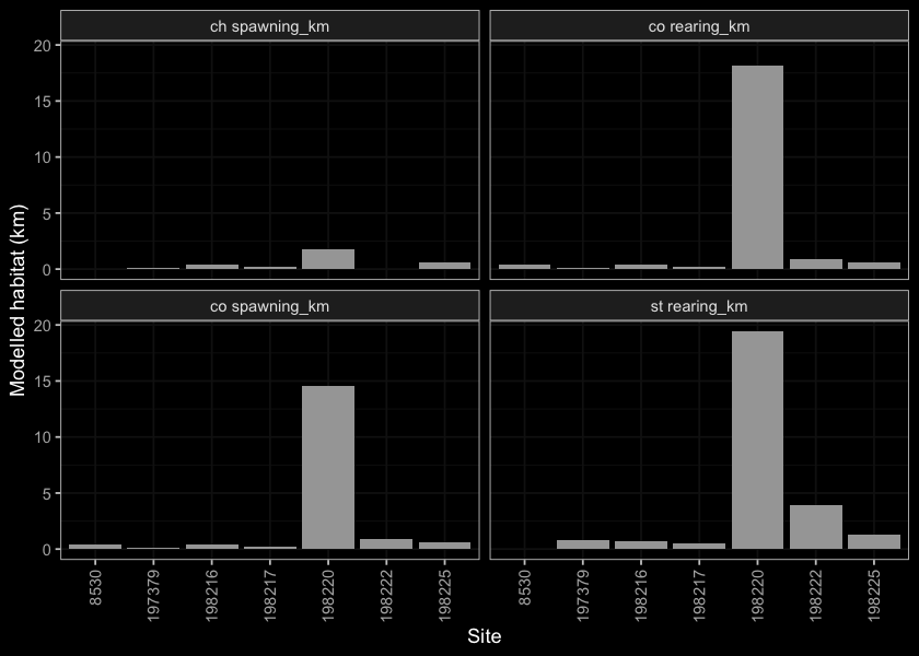
Figure 4.2: Summary of potential habitat upstream of habitat confirmation assessment sites estimated based on modelled channel width and upstream channel length.
4.2.1 Fish Sampling
Fish sampling was conducted at 8 sites with a total of 146 fish captured. Fork length data was used to delineate salmonids based on life stages: fry (0 to 65mm), parr (>65 to 110mm), juvenile (>110mm to 140mm) and adult (>140mm) by visually assessing the histograms presented in Figure 4.3. A summary of sites assessed are included in Table 4.7 and raw data is provided in Attachment 3. A summary of density results for all life stages combined of select species is also presented in Figure 4.4. Results are presented in greater detail within individual habitat confirmation site appendices.
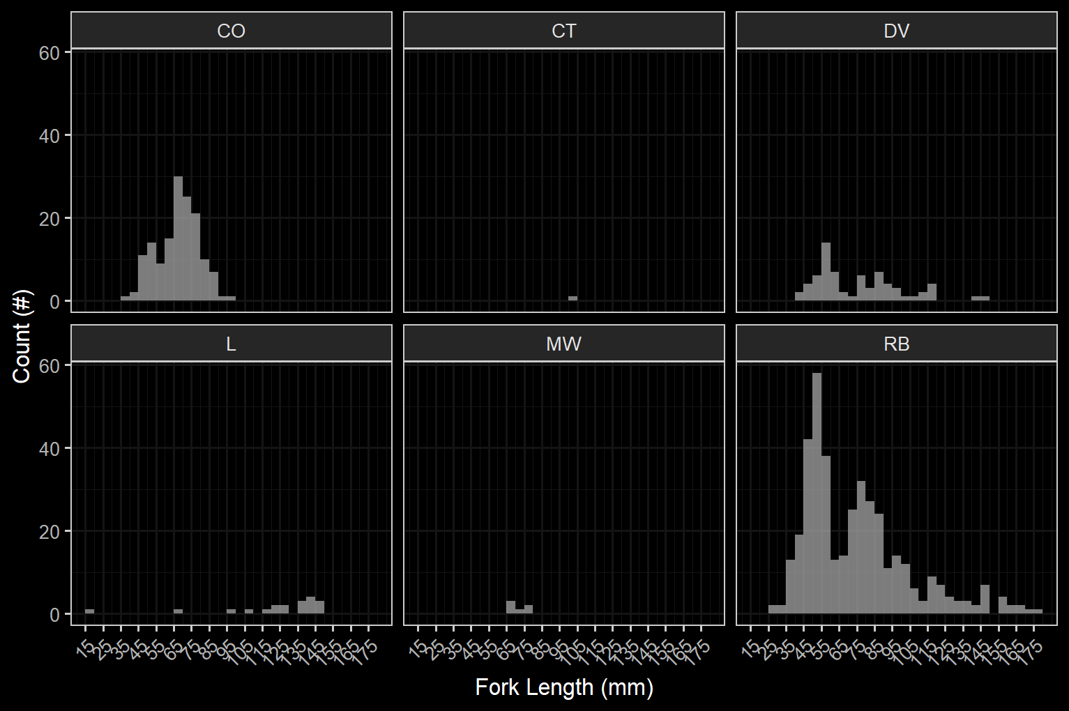
Figure 4.3: Histograms of fish lengths by species. Fish captured by electrofishing during habitat confirmation assessments.
tab_fish_sites_sum %>%
fpr::fpr_kable(caption_text = 'Summary of electrofishing sites.', scroll = F)| site | passes | ef_length_m | ef_width_m | area_m2 | enclosure |
|---|---|---|---|---|---|
| 197379_ds_ef1 | 1 | 5 | 5.00 | 25.0 | Open |
| 197379_us_ef1 | 1 | 11 | 1.70 | 18.7 | Open |
| 8530_ds_ef1 | 1 | 14 | 2.40 | 33.6 | Open |
| 8530_ds_ef2 | 1 | 15 | 3.33 | 50.0 | Open |
| 8530_ds_ef3 | 1 | 11 | 4.15 | 45.7 | Open |
| 8530_us_ef1 | 1 | 17 | 2.40 | 40.8 | Open |
| 8530_us_ef2 | 1 | 21 | 2.40 | 50.4 | Open |
| 8530_us_ef3 | 1 | 21 | 2.80 | 58.8 | Open |
plot_fish_box_all <-  fish_abund %>% #tab_fish_density_prep
    filter(
      !species_code %in% c('MW', 'SU', 'NFC', 'CT', 'LSU')
    ) %>%
    ggplot(., aes(x = location, y =density_100m2)) +
    geom_boxplot()+
    facet_grid(site ~ species_code, scales ="fixed", #life_stage
               as.table = T)+
    # theme_bw()+
    theme(legend.position = "none", axis.title.x=element_blank()) +
    geom_dotplot(binaxis='y', stackdir='center', dotsize=1)+
    ylab(expression(Density ~ (Fish/100 ~  m^2))) +
    ggdark::dark_theme_bw()

plot_fish_box_all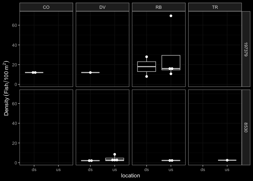
Figure 4.4: Boxplots of densities (fish/100m2) of fish captured by electrofishing during habitat confirmation assessments.
4.3 Engineering Design - Phase 3
Engineering designs have been completed for replacement of PSCIS crossing 58159 on McDowell Creek (Irvine 2021) with a clear-span bridge and for removal of the collapsed bridge (PSCIS crossing 197912) on Robert Hatch Creek. Designs for McDowell and Robert Hatch were procured by SERNbc and Canadian Wildlife Federation respectively. At the time of reporting, the Ministry of Transportation and Infrastructure, in collaboration with Canadian Wildlife Federation was in the process of procuring designs for remediation of fish passage at three sites documented in Irvine (2021) including PSCIS 123445 on Tyhee Creek, PSCIS 124500 on Helps Creek and PSCIS 197640 on a tributary to Buck Creek. Additionally, the Ministry of Transportation and Infrastructure were procuring a design for PSCIS crossing 124420 on Station Creek (also know as Mission Creek) near New Hazleton (pers. comm. Sean Wong, Environmental Programs, MoTi).
4.4 Climate Change Risk Assessment
Preliminary climate change risk assessment data for Ministry of Transportation and Infrastructure sites is presented below. Phase 1 sites are contained in Table 4.8, and Phase 2 sites are in Table 4.9. Raw data is provided here.
source('scripts/moti_climate.R')

df_transpose <- function(df) {

  df %>%
    tidyr::pivot_longer(-1) %>%
    tidyr::pivot_wider(names_from = 1, values_from = value)

}

tab_moti_phase1 %>%
  select(-contains('Describe'), -contains('Crew')) %>%
  rename(Site = pscis_crossing_id,
         'External ID' = my_crossing_reference,
         `MoTi ID` = moti_chris_culvert_id,
         Stream = stream_name,
         Road = road_name) %>%
  mutate(across(everything(), as.character)) %>%
  tibble::rownames_to_column() %>%
  df_transpose() %>%
  janitor::row_to_names(row_number = 1) %>%
  fpr::fpr_kable(scroll = gitbook_on,
caption_text = 'Preliminary climate change risk assessment data for Ministry of Transportation and Infrastructure sites (Phase 1 PSCIS)')| Site | 198200 | 198215 | 198216 | 198197 | 198209 | 198206 | 198186 | 198221 | 198196 | 198202 | 198201 | 198207 |
|---|---|---|---|---|---|---|---|---|---|---|---|---|
| External ID | 8300012 | 8300042 | 8300054 | 8300105 | 8300111 | 8300118 | 8300162 | 8300178 | 8300186 | 8300188 | 8300917 | 2022090501 |
| MoTi ID | 1528424 | 1524776 | 3321227 | 3321236 | 1524149 | 1525645 | 1524552 | 1529688 | 1524780 | 1529371 | 1528426 | 1524566 |
| Stream | Tea Creek | Dale Creek | Tributary to Skeena River | Tributary to Kispiox River | Tributary to Kispiox River | Tributary to McCully Creek | Tributary to Kispiox River | Tributary to Kitwanga River | Tributary to Kispiox River | Tributary to Kitwanga River | Tributary to Tea Creek | Tributary to Kispiox River |
| Road | Moore Road | Date Creek FSR | Kispiox Valley Road | Kispiox Valley Road | Kispiox Valley Road | Helen Lake Road | Poplar Park Road | 11A Ave | Date Creek FSR | Hwy 37 | Moore Road | Poplar Park Rd |
| Erosion (scale 1 low - 5 high) | 1 | 1 | 1 | 2 | 1 | 1 | 1 | 1 | 2 | 1 | 3 | 1 |
| Embankment fill issues 1 (low) 2 (medium) 3 (high) | 1 | 1 | 1 | 1 | 1 | 1 | 1 | 1 | 1 | 1 | 2 | 1 |
| Blockage Issues 1 (0-30%) 2 (>30-75%) 3 (>75%) | 1 | 2 | 2 | 1 | 1 | 1 | 2 | 2 | 1 | 1 | 1 | 2 |
| Condition Rank = embankment + blockage | 3 | 4 | 4 | 4 | 3 | 3 | 4 | 4 | 4 | 3 | 6 | 4 |
| Likelihood Flood Event Affecting Culvert (scale 1 low - 5 high) | 1 | 1 | 1 | 2 | 1 | 1 | 1 | 4 | 1 | 3 | 2 | 1 |
| Consequence Flood Event Affecting Culvert (scale 1 low - 5 high) | 1 | 3 | 4 | 2 | 3 | 1 | 1 | 1 | 1 | 5 | 2 | 3 |
| Climate Change Flood Risk (likelihood x consequence) 1-6 (low) 6-12 (medium) 10-25 (high) | 1 | 3 | 4 | 4 | 3 | 1 | 1 | 4 | 1 | 15 | 4 | 3 |
| Vulnerability Rank = Condition Rank + Climate Rank | 4 | 7 | 8 | 8 | 6 | 4 | 5 | 8 | 5 | 18 | 10 | 7 |
| Traffic Volume 1 (low) 5 (medium) 10 (high) | 3 | 3 | 8 | 5 | 5 | 1 | 4 | 1 | 7 | 9 | 5 | 1 |
| Community Access - Scale - 1 (high - multiple road access) 5 (medium - some road access) 10 (low - one road access) | 8 | 3 | 10 | 7 | 5 | 5 | 8 | 1 | 9 | 8 | 9 | 1 |
| Cost (scale: 1 high - 10 low) | 8 | 5 | 2 | 4 | 7 | 1 | 7 | 1 | 6 | 2 | 8 | 10 |
| Constructibility (scale: 1 difficult -10 easy) | 9 | 5 | 2 | 6 | 7 | 10 | 8 | 9 | 5 | 4 | 8 | 10 |
| Fish Bearing 10 (Yes) 0 (No) - see maps for fish points | 10 | 10 | 10 | 10 | 0 | 0 | 0 | 10 | 0 | 0 | 10 | 0 |
| Environmental Impacts (scale: 1 high -10 low) | 7 | 7 | 9 | 6 | 1 | 10 | 8 | 9 | 6 | 4 | 7 | 10 |
| Priority Rank = traffic volume + community access + cost + constructability + fish bearing + environmental impacts | 45 | 33 | 41 | 38 | 25 | 27 | 35 | 31 | 33 | 27 | 47 | 32 |
| Overall Rank = Vulnerability Rank + Priority Rank | 49 | 40 | 49 | 46 | 31 | 31 | 40 | 39 | 38 | 45 | 57 | 39 |
source('scripts/moti_climate.R')

df_transpose <- function(df) {

  df %>%
    tidyr::pivot_longer(-1) %>%
    tidyr::pivot_wider(names_from = 1, values_from = value)

}

tab_moti_phase2 %>%
  purrr::set_names(nm = xref_moti_climate %>% pull(report)) %>%
  select(-my_crossing_reference) %>%
  select(-contains('Describe'), -contains('Crew')) %>%
  rename(Site = pscis_crossing_id,
         `MoTi ID` = moti_chris_culvert_id,
         Stream = stream_name,
         Road = road_name) %>%
  mutate(across(everything(), as.character)) %>%
  tibble::rownames_to_column() %>%
  df_transpose() %>%
  janitor::row_to_names(row_number = 1) %>%
  fpr::fpr_kable(scroll = gitbook_on,
caption_text = 'Preliminary climate change risk assessment data for Ministry of Transportation and Infrastructure sites (Phase 2 PSCIS)')| Site | 198215 | 198216 | 198220 |
|---|---|---|---|
| MoTi ID | 1524776 | 3321227 | 4092 |
| Stream | Tributary to Kispiox River | Tributary to Skeena River | Tea Creek |
| Road | Date Creek FSR | Kispiox Valley Road | Highway 37 |
| Erosion (scale 1 low - 5 high) | 1 | 1 | 3 |
| Embankment fill issues 1 (low) 2 (medium) 3 (high) | 1 | 1 | 1 |
| Blockage Issues 1 (0-30%) 2 (>30-75%) 3 (>75%) | 2 | 2 | 1 |
| Condition Rank = embankment + blockage | 4 | 4 | 5 |
| Likelihood Flood Event Affecting Culvert (scale 1 low - 5 high) | 1 | 1 | 1 |
| Consequence Flood Event Affecting Culvert (scale 1 low - 5 high) | 3 | 4 | 5 |
| Climate Change Flood Risk (likelihood x consequence) 1-6 (low) 6-12 (medium) 10-25 (high) | 3 | 4 | 5 |
| Vulnerability Rank = Condition Rank + Climate Rank | 7 | 8 | 10 |
| Traffic Volume 1 (low) 5 (medium) 10 (high) | 3 | 8 | 9 |
| Community Access - Scale - 1 (high - multiple road access) 5 (medium - some road access) 10 (low - one road access) | 3 | 10 | 1 |
| Cost (scale: 1 high - 10 low) | 5 | 2 | 1 |
| Constructibility (scale: 1 difficult -10 easy) | 5 | 2 | 2 |
| Fish Bearing 10 (Yes) 0 (No) - see maps for fish points | 10 | 10 | 10 |
| Environmental Impacts (scale: 1 high -10 low) | 7 | 9 | 2 |
| Priority Rank = traffic volume + community access + cost + constructability + fish bearing + environmental impacts | 33 | 41 | 25 |
| Overall Rank = Vulnerability Rank + Priority Rank | 40 | 49 | 35 |